

Recently I read some articles about the Hill of Value. I’m not going into detail about it but the Hill of Value is a mine optimization approach that’s been around for a while. Here is a link to an AusIMM article that describes it “The role of mine planning in high performance”. For those interested, here is a another post about this subject “About the Hill of Value. Learning from Mistakes (II)“.
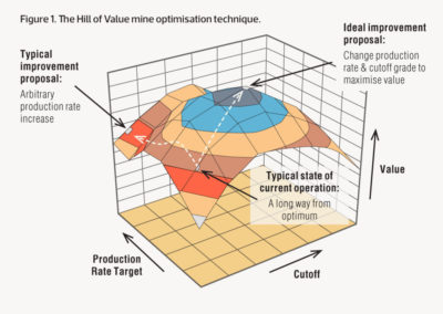
(From AusIMM)
The basic premise is that an optimal mining project is based on a relationship between cut-off grade and production rate. The standard breakeven or incremental cutoff grade we normally use may not be optimal for a project.
The image to the right (from the aforementioned AusIMM article) illustrates the peak in the NPV (i.e. the hill of value) on a vertical axis.
A project requires a considerable technical effort to properly evaluate the hill of value. Each iteration of a cutoff grade results in a new mine plan, new production schedule, and a new mining capex and opex estimate.
Each iteration of the plant throughput requires a different mine plan and plant size and the associated project capex and opex. All of these iterations will generate a new cashflow model.
The effort to do that level of study thoroughly is quite significant. Perhaps one day artificial intelligence will be able to generate these iterations quickly, but we are not at that stage yet.
Can we simplify it?
In previous blogs (here and here) I described a 1D cashflow model that I use to quickly evaluate projects. The 1D approach does not rely on a production schedule, instead uses life-of-mine quantities and costs. Given its simplicity, I was curious if the 1D model could be used to evaluate the hill of value.
I compiled some data to run several iterations for a hypothetical project, loosely based on a mining study I had on hand. The critical inputs for such an analysis are the operating and capital cost ranges for different plant throughputs.
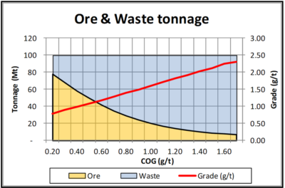 I had a grade tonnage curve, including the tonnes of ore and waste, for a designed pit. This data is shown graphically on the right. Essentially the mineable reserve is 62 Mt @ 0.94 g/t Pd with a strip ratio of 0.6 at a breakeven cutoff grade of 0.35 g/t. It’s a large tonnage, low strip ratio, and low grade deposit. The total pit tonnage is 100 Mt of combined ore and waste.
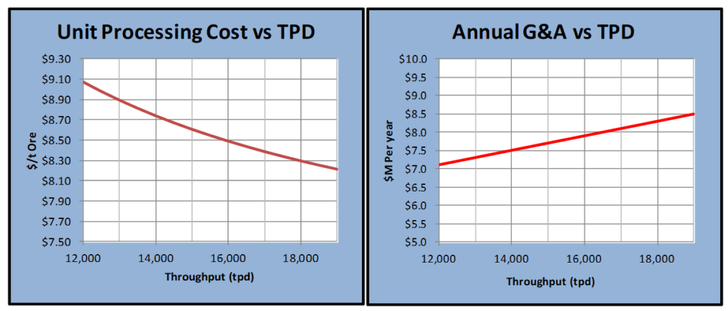
I estimated capital costs and operating costs for different production rates using escalation factors such as the rule of 0.6 and the 20% fixed – 80% variable basis. It would be best to complete proper cost estimations but that is beyond the scope of this analysis. Factoring is the main option when there are no other options.
The charts below show the cost inputs used in the model. Obviously each project would have its own set of unique cost curves.
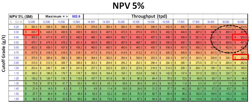
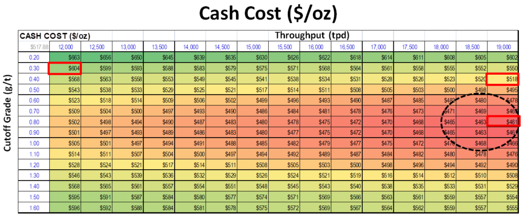
The 1D cashflow model was used to evaluate economics for a range of cutoff grades (from 0.20 g/t to 1.70 g/t) and production rates (12,000 tpd to 19,000 tpd). The NPV sensitivity analysis was done using the Excel data table function. This is one of my favorite and most useful Excel features.
A total of 225 cases were run (15 COG versus x 15 throughputs) for this example.

What are the results?
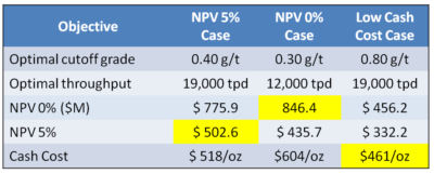
The results are shown below. Interestingly the optimal plant size and cutoff grade varies depending on the economic objective selected.
The discounted NPV 5% analysis indicates an optimal plant with a high throughput (19,000 tpd ) using a low cutoff grade (0.40 g/t). This would be expected due to the low grade nature of the orebody. Economies of scale, low operating costs, high revenues, are desired. Discounted models like revenue as quickly as possible; hence the high throughput rate.
The undiscounted NPV 0% analysis gave a different result. Since the timing of revenue is less important, a smaller plant was optimal (12,000 tpd) albeit using a similar low cutoff grade near the breakeven cutoff.
If one targets a low cash cost as an economic objective, one gets a different optimal project. This time a large plant with an elevated cutoff of 0.80 g/t was deemed optimal.
The Excel data table matrices for the three economic objectives are shown below. The “hot spots” in each case are evident.

Conclusion
 The Hill of Value is an interesting optimization concept to apply to a project. In the example I have provided, the optimal project varies depending on what the financial objective is. I don’t know if this would be the case with all projects, however I suspect so.