Mining’s Obsession with Optimization – Good or Bad?

Date: March 31, 2026 Author: Ken Kuchling Comments: Leave a reply

You read a lot these days about the push for more optimization in mining. Ore grades are declining and high-grade, easy-to-process deposits are becoming scarcer, forcing new projects to face greater risk. To compensate for this, miners are told to optimize and innovate more. They are doing both; including making technological gains.

Mining has gotten better at squeezing more value from each tonne of ore. So why do see mining projects still stumbling and everyone being pushed to do even more optimization?

The answer may be that the industry is confusing optimization with resilience. A mine tuned to perform perfectly under one set of conditions may become fragile when those conditions shift. And in mining, things are always shifting. Maybe the head grades don’t meet expectations or metal prices collapse. Maybe there is a shift in community sentiment or a geotechnical surprise in the mine.

The pursuit of a single “optimal” outcome might leave projects well engineered, yet poorly equipped for reality. Flexibility (or resiliency) aren’t the enemy of efficiency; they may be the only way to make efficiency sustainable.

Which Aspects Should Be Optimized

Is the concept of optimization the most important factor in a project’s design? If so, which aspect is the most important to optimize? A danger is optimizing for a single criteria, for example NPV, at the expense of everything else. Selecting the optimal design for one aspect will likely result in being sub-optimal in some of the others.

Once one has selected the aspect to optimize, the next issue becomes what to base the optimization on. Optimization typically is founded on a specific set of inputs. When these change, the optimized design will likely require revision. This then forces a new optimization, which can create a never-ending optimization loop because things are always changing in mining.

The design aspects that I have seen recommended for optimization range from:

optimize your drill hole locations
optimize your pit size
optimize your production schedule
optimize your throughput and/or recovery
optimize your water consumption
optimize your carbon footprint
optimize your project design
optimize your labour productivity
optimize either NPV, IRR, or payback
optimize your metal production cash cost

There are a lot of suggestions and recommendations and people will have differing opinion on which are the most important optimizations. This opinion is typically driven by their own expertise or field of work, not necessarily by what is best for the project.

Optimal vs Resilient Design

Optimization of a mining project can yield meaningful cost and efficiency gains. However mines face inherent constraints, such as ore grade variability, geological surprises, equipment life cycles, and regulatory issues.

Company success is typically driven by a broader set of variables: commodity price cycles, capital availability, asset portfolio quality, ESG and social license, M&A timing, and balance sheet strength. A perfectly optimized mine in a declining commodity or in a politically unstable jurisdiction may underperform a less-optimized mine in the right location at the right time.

Chasing optimization can sometimes lead to over-investment in a single asset, reduced flexibility, or operational fragility. The system performs well only under the ideal conditions.

Hence flexibility is important. If the mine plan is so rigid that it cannot pivot when a new high-grade zone is discovered or a pit wall becomes unstable, then one has optimized for a single scenario rather than for long-term resilience. Rather than designing for the “best case,” design for resilience.

Flexibility builds in the ability to scale production up or down, switch mining sequences, or pivot processing approaches as conditions change. Resilience has real value in mining, where geology, markets, and costs are unpredictable.

Flexibility identifies and can mitigate technical, geopolitical, regulatory, environmental, and market risks. The mines that do run into trouble rarely do so because they weren’t optimized; they fail because key risks weren’t anticipated or managed.

Workforce capability, safety culture, and leadership quality are key predictors of operational success. Optimization alone may not be able to address high turnover, poor safety records, and weak supervisory capacity. These can erode profitability far more than sub-optimal scheduling.

In my experience, the best operations have systems for ongoing learning and improvement rather than seeking a one-time optimal design. However, there is still a place for full optimization in some situations.

When does a flexible project design win?

Commodity prices are volatile up and down
Geological uncertainty is high (low proportion of Measured Resource)
Mining uncertainty (limited geotechnical investigations)
Long mine life (10–30+ years), where conditions will certainly change
Regulatory or social environments are unpredictable
Capital markets may require staged investment rather than full financing

When does an optimal project design win?

Shorter mine life where conditions are unlikely to change materially
Commodity is stable, well-hedged, or under long term offtake contract pricing
Geology and processability is well-understood (mature, well drilled-out deposit)
Capital is constrained and upfront efficiency is critical (you need to get it right)

Unfortunately some might view flexibility as a weakness. If a company has to change a plan or pivot, some will view that as a sign that the company is poor at planning and they don’t know what they are doing. In some cases, this might be true. Conversely the company may simply be reacting to unforeseeable outside influences.

The Path to Resiliency

If one decides to pursue the path of operational flexibility, what are the things that help make it happen?

Design for flexibility at the start: Build project components that can scale up or down as needed. This might include wider pit ramps, larger infrastructure, some modularization in the processing system and the mine. Building a single rigid optimal design can be a trap. Open pit mines may be inherently more flexible than underground mines.
Maintain multiple ore sources: Maintain flexibility across different mining areas and ore zones with different metallurgy or head grades means one can blend ore as needed. Multiple mining areas provide flexibility in the case of geotechnical or weather events. Multiple stockpiling is also part of flexibility in design and operation.
Be careful consuming all high grade ore: In order to boost NPV, often most of the high grade ore is consumed early in the schedule, meaning the back part of the schedule relies on low grade material. This reduces economic flexibility if prices decrease in the future and may also miss out on the benefits if prices rise.
Real-time data collection and adaptive planning: Real time control systems let operations respond to actual conditions rather than following a fixed weekly plan. The idea is to shorten the time between observation and reaction, not to automate rigidly but enable the system to adapt rapidly.
Keep a cross-trained workforce: Operational flexibility may be enhanced if people can fill multiple roles. Cross-training operators means one can redeploy people as needed when conditions change.
Maintain financial health: A company with low debt, high cash assets, and easy credit access can keep a mine on basic functionality (or care-and-maintenance) rather than being forced to sell assets or close the doors during a downturn. Financial health will help ensure operational flexibility. The major miners already know this. The junior miners learn it the hard way.
Build supplier and contractor relationships before needed: Much like access to credit, long-term supplier arrangements might mean one can find labor and materials faster than competitors scrambling during downturns or upturns.
Scenario-plan continuously: Run multiple what-if commodity price, head grade, geotechnical & water management scenarios regularly during operations, not just at the feasibility or permitting stage. Operations change over time, and teams that have already pre-planned “what if this happens” respond better when it really happens.

Flexible mining operations may sacrifice a little efficiency at peak conditions and not meet the fully optimized vision. However this flexibility is a trade-off for the ability to stay profitable over a range of scenarios.

Conclusion

Rather than focus on constant optimization in design, it may be wiser to focus on a flexible design. Adaptability, flexibility, and resilience may be more important than being fully optimized.

Modern mine planning is starting to consider Real Options Analysis and stochastic optimization (Monte Carlo simulation) to help quantify the value of flexibility. They may find that a slightly suboptimal design is actually worth more than a rigid optimized one when uncertainty is priced in.

Probabilistic analysis can provide some assistance by highlighting the impact of unforeseen events. However the key is not just to know the event’s impact, but also how will one respond even if there is only a 10% probability of it occurring.

Optimization may be great, but it isn’t everlasting. Squeezing the last dollar out of a plan may be less important than keeping a mine in business. A flexible plan may actually be the optimal plan.

end

In case you missed it, the last blog post was “The Surprising Parallels Between Junior Miners and Tech Startups“. The entire blog post library can be found at https://kuchling.com/library/

You can sign up for the KJK mailing list to get notified when new blogs are posted. Follow me on Twitter at @KJKLtd for updates and other mining posts.

Beyond the Headline Grade: For or Against Assay Transparency?

Date: March 11, 2026 Author: Ken Kuchling Comments: Leave a reply

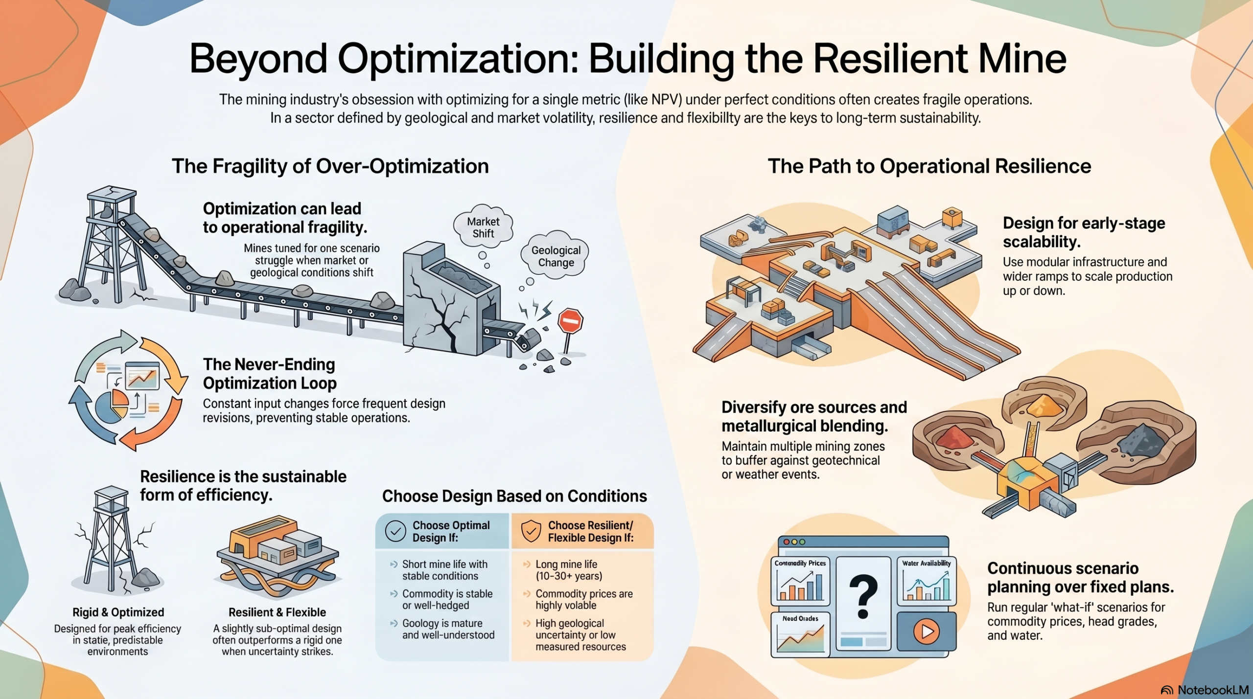
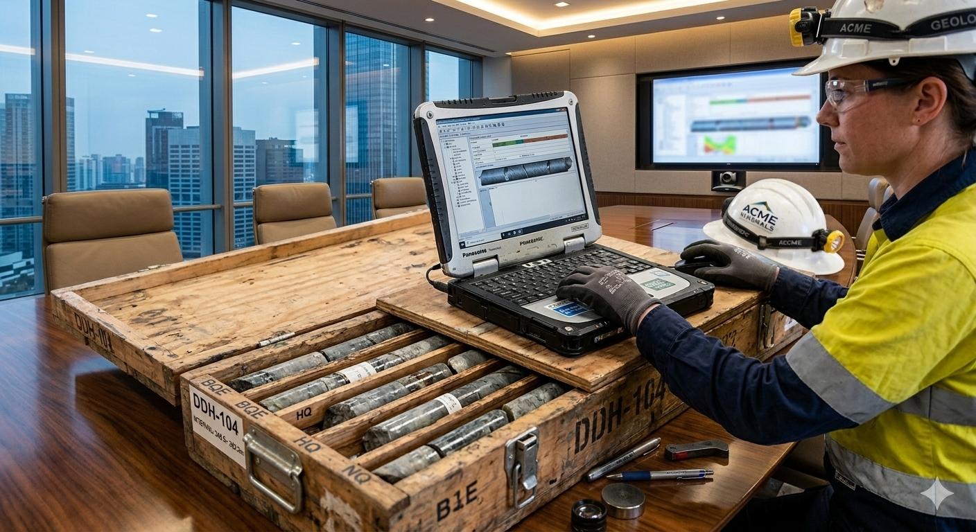
Recently I have been reviewing a few mining projects from an investor’s perspective. This led me to wonder whether junior mining companies should share more than just their drill hole highlights. What about the raw assays? A mining company announces highlighted drill intervals, but what exactly do those numbers represent?

The highlighted drill interval is based on a series of individual assay samples. The selection of the interval “From” and “To” and “Including” is made by the company using their own criteria. They may include low-grade sections (i.e. smoothing), apply variable cutoffs, sometimes use metal equivalent grades or NSR value to defines the ore/waste cutoff.

The interval definition process is largely invisible to investors, yet for early-stage projects, drill hole intervals are the primary driver of investor communications and their own project valuation.

The underlying basis for drill intervals are raw assay data. These assays can be complex, messy, technical, and may require expertise to interpret properly. However examining the individual assay data can tell more of the story than looking at intervals alone. For example, assays will demonstrate the grade continuity, any nugget effects, or whether thin high-grade spikes are boosting average grades.

This raises the question of whether companies should routinely publish, in CSV format, for download BOTH interval data and raw assay data.

This blog post discusses the pros and cons of releasing assay data electronically.

Why Might an Investor Want the CSV Data

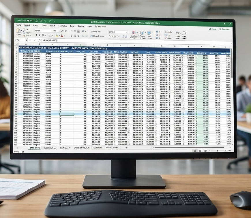
There is a sense that many mining investors are becoming more sophisticated, and they want to fully understand the exploration process.

Some investors have geological software with which to examine the exploration data in 3D. Other investors may simply rely on Excel to run their own statistics. Investors may wish to verify what a company is doing, as well as examine their own concept for a project.

Investors might be questioning whether:

Companies change the nature of a deposit by smoothing narrow high grade intervals over wider intervals to give the impression of a large tonnage bulk deposit;
Companies are using by-product metals in their metal-equivalent, which investors have less confidence in. Perhaps they would prefer to examine the deposit based solely on their primary metals of interest. Perhaps investors prefer to understand the NSR Rock Value ($/t) instead of relying metal-equivalent grades.
Companies have not provided sufficient geological cross-sections or 3D images, and investors wish to create their own.

To examine any of these issues, one must have the exploration data in electronic format. For large players, signing an NDA (Non-Disclosure Agreement) and entering the corporate data room provides preferential access to this information. Small players may not be able to do this and some may consider this unfair and selective disclosure.

Highlighted Interval Data in CSV Format

Companies will disclose all highlighted drill INTERVALS in news releases, usually in table format (see example image). If someone wishes to analyze all the interval data on a project, it can be a tedious process to gather all the new releases PDF’s. The tabular data can then be scraped using Ai or one can use Excel “Get Data” functionality on a table by table basis.

This work can be cumbersome and sometimes data does not transform cleanly, often with missing rows, columns, or misaligned data.

Why make investors jump though those hoops to summarize data that’s already been disclosed? Hence, I would suggest companies maintain downloadable historical drill interval data in CSV format on their websites, in a format as presented in the news releases.

Raw assay data, however, is a different matter than interval data since assays have not been made public in the news releases. This is discussed in the next section.

Raw Assay Data in CSV Format

Deciding whether to release raw drill hole assay data is a balance between transparency and strategic risk. The only companies that are doing this (that I am aware of) is Power Metallic and (previously) Great Bear Resources. There may be more that i am not privy to.

There are both pros and cons to making the raw assay data available. Note that raw assay data files typically will also include drill hole collar coordinates and downhole survey information, the whole package.

The Pro’s and Benefits of Raw Data Disclosure

1. Market Credibility: A company being “radically transparent” can set them apart by signaling to the market confidence in their data and they have nothing to hide. This can build trust with those who want to verify the discovery. This can differentiate one from peers in a crowded junior market where transparency may be lacking.

2. Free Technical Analysis: Raw data appeals to technically sophisticated investors, geologists, and analysts who want to do their own review. The independent “super-investors” who run their own models may reach the same conclusions as the company, proving external validation for the project. They may essentially help IR with free marketing and 3rd party promotion. Of course, the opposite can also happen if the project is not as robust as being promoted by the company.

3. Speed: Raw data access may speed up due diligence for potential acquirers or JV partners who can initiate confidential internal reviews prior to deciding whether to enter a formal NDA and due diligence process.

The Con’s and Risks of Raw Data Disclosure

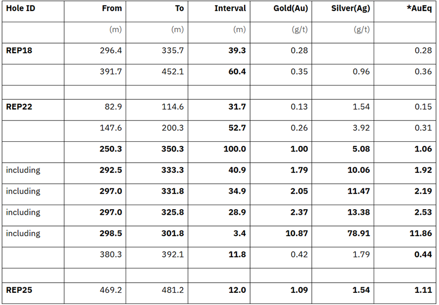
1. Misinterpretation & “Amateur” Experts: One risk is that someone with a very basic understanding of mining software and limited understanding of the local geology, runs flawed interpretations and publicizes their incorrect conclusions. A company may find that correcting false narratives publicly can be harder than preventing them.

Conversely stock pumpers can cherry-pick individual high-grade intervals out of context and also create misleading narratives (albeit positive) outside of the company control. They may have their own motives to pump the stock.

2. Competitive Intelligence: If in a competitive exploration district, neighbors can use raw assay values and lithology codes to predict where the mineralization is trending. This could help them acquire adjacent mineral claims before one can fully consolidate the regional land package. Regardless, competitors may still be able to do some of this using the drill hole interval data from news releases, so this may not be a big risk.

3. Liability and Compliance: NI 43-101 reporting requires technical data to be verified by a Qualified Person (QP). If one provides a raw assay file that isn’t properly vetted or contains errors, will there be regulatory or legal issues? Normally a corporate QP signs off on news releases, not necessarily an independent QP.

There have also been cases where assay data has been purposely manipulated from lab certificates to the drill hole database, and investors would then be working with this falsified data. Corporate liability could be a big risk in the eyes of some.

The Assay Disclosure Middle Ground

Once the assay data is public, it may be more difficult for a company to manage the story. A press release lets them frame results in the context of their business plan; a raw data file does not.

Instead of providing a full assay database download, some companies might follow the approach below. It may not satisfy everyone, but could be better than just ignoring requests for more detailed information.

Interactive Map: Use a web-based GIS tool that allows users to click holes and see downhole results graphically without downloading the full database.
Cross-Sections: Provide multiple high-quality cross-sections that show the geological interpretation alongside the raw assay grades or use a grade bar chart along the drill hole trace. This provides information on the grade continuity and uniformity without releasing the actual grades.
Post-resource estimate disclosure: Once the database has been formally audited by an independent QP and incorporated into a 43-101 technical report for a resource estimate, releasing the assay data may be lower risk.

These actions may give a sense of greater transparency while keeping the raw data within a controlled environment. It will help prevent amateurs from erroneous modeling the geology yet still “somewhat” satisfying the sophisticated mining investor.

Conclusion

For investors trying to assess a junior explorer, or geologists conducting a technical review, or a regulator trying to ensure fair and accurate disclosure, access to raw assay data can play a part in promoting good judgment and accurate disclosure from companies.

However some suggest that raw data without context is subject to misinterpretation.

Personally, I would prefer to see the release of both drill intervals and raw assay tables in CSV format.

In this modern area of Ai and investor sophistication, greater data transparency may be a positive and help build more trust in the industry. However, I understand the reasons not to do this and understand if companies choose to not go this route.

Currently the mining industry norm is that raw assays stay in private data rooms and not on corporate websites. Credibility tries to be achieved via clear, technically detailed news releases and Technical Reports.

In case you missed it, the last blog post was “What Does Ai Think of Toll Milling“.

You can sign up for the KJK mailing list to get notified when new blogs are posted. Follow me on Twitter at @KJKLtd for updates and other mining posts. The entire blog post library can be found at https://kuchling.com/library/

APPENDIX: EXCEL TASKS with and ASSAY DATABASE

I asked an Ai colleague Claude to list all the things one could do in Excel with publicly released drill hole information. Here is what it said (unedited). Its never lacking in advice and Claude will even help you create the Excel worksheet logic if needed.

Grade Analysis

Descriptive statistics – mean, median, mode, min/max, standard deviation of assay values (Au, Ag, Cu, etc.)

Grade frequency distributions — histogram charts to understand grade population shape.
High-grade outlier identification — flagging values above a threshold (e.g., >3x median) that may need capping consideration.
Grade capping/cutting analysis — testing different cap values and their effect on average grade.
Coefficient of Variation (CV) — assessing grade variability and nugget effect risk.

Composite & Interval Analysis

Downhole compositing — averaging assay intervals into fixed-length composites (e.g., 2m or 5m) using weighted averages.
True width estimation — applying trigonometric corrections for hole dip/azimuth vs. vein orientation.

Grade x thickness (GT) calculations — multiplying average grade by intercept width for comparative ranking of intersections.
Cut-off grade sensitivity — running intercept calculations at multiple cut-off grades to see how reported widths and grades change.

Hole Correlation & Comparison

Hole-by-hole grade comparison — ranking holes by peak grade, average grade, or GT value.
Section-by-section comparison— grouping holes by fence/section for along-strike trend analysis.
Depth vs. grade plots — scatter plots to look for grade zonation with depth.
Multi-element ratio analysis— e.g., Au:Ag ratios, Cu:Mo ratios to identify metallogenic zonation or alteration trends.

Spatial & Trend Analysis

Collar location plotting — basic X/Y scatter plots of collar coordinates to visualize drill pattern coverage.
Downhole survey data — using dip/azimuth measurements to approximate downhole trace (basic desurveying).
Strike and dip trend identification — plotting grade against easting or northing to identify directional trends.
Variogram-lite analysis — plotting grade vs. distance between holes to get a rough sense of spatial continuity (proper variography needs dedicated software).

Multi-Element & Geochemical Analysis

Correlation matrices — identifying which elements are positively or negatively correlated (e.g., Au vs. As in a Carlin-type system).
Scatter plots — visualizing element-pair relationships to identify pathfinder associations.
Log-transformation — applying LOG10 to skewed assay data before statistical analysis, which is standard practice.
Anomaly thresholding— mean + 2 standard deviations as a simple anomaly threshold for pathfinder elements.

Resource Estimation (Basic)

Polygonal area calculations — basic area-of-influence resource estimation using drill spacing geometry.
Grade tonnage curves — plotting tonnes vs. grade at varying cut-offs using simplified volume assumptions.
Bulk density sensitivity** — testing how different SG assumptions affect tonnage estimates.

Reporting & QA/QC

Duplicate analysis — comparing field duplicate, coarse reject duplicate, and pulp duplicate pairs using scatter plots and % relative difference calculations.
Standard performance tracking — plotting certified reference material (CRM) results against expected values and control limits (±2SD, ±3SD).
Blank monitoring — flagging blank samples that exceed contamination thresholds.
Laboratory turnaround tracking — monitoring submission dates vs. return dates.

Mine Reconciliation – Standardization Please

Date: May 7, 2025 Author: Ken Kuchling Comments: Leave a reply

Mine through mill reconciliation, in my view, is an under appreciated topic that could benefit from more conversation amongst industry members. Unfortunately, reconciliation is sometimes viewed as a time consuming frustrating activity, with what some consider less than verifiable results. However given the ongoing innovation that we are seeing in mining, reconciliation may need to play a bigger role than ever.

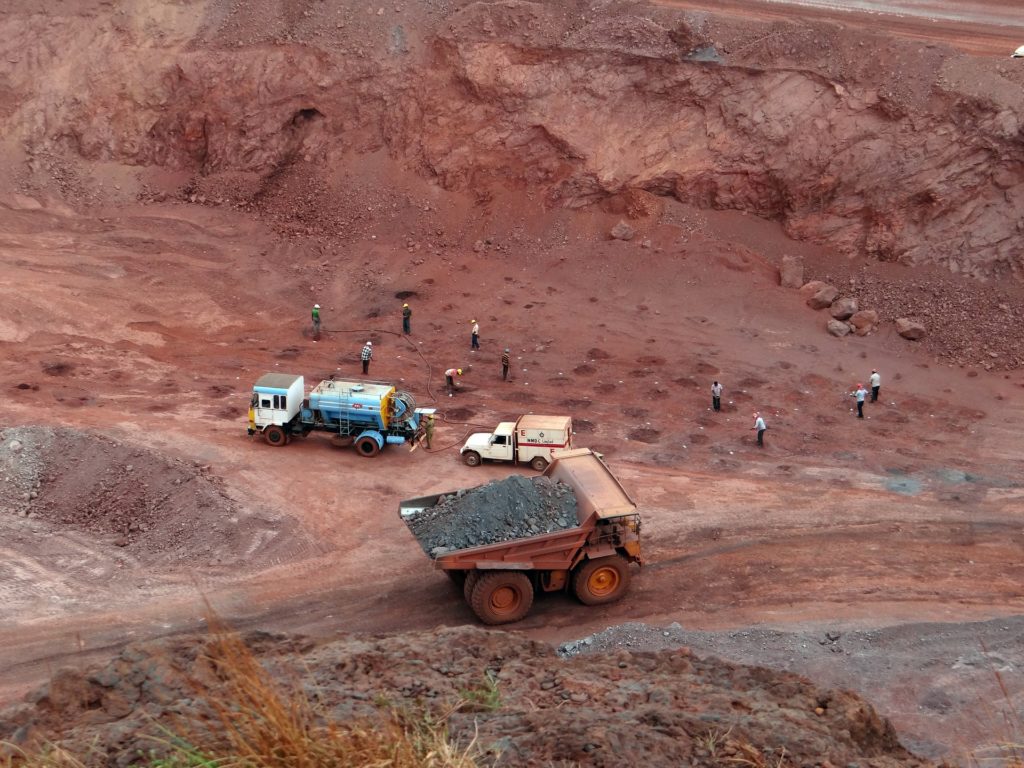
The mining industry is implementing more and more technology in the mining cycle.

For example, this can range from AI assisted resource modelling, down hole logging, blast movement tracking, GPS controlled dig limits, MineSense bucket grade tracking, load scanning, truck dispatch control, smart mining and edge computing, online grade analyzers, belt weightometers, drone surveying of stockpiles, and real time process controls.

Lots of different innovations are continually being adopted by the mining industry, contrary to what some may say.

The question is does all this innovation improve the overall performance of a mining operation, and if so, by how much? It can cost a lot of money to implement the new technology, is there a payoff?

One cannot answer those questions if one doesn’t undertake proper mine reconciliation. A concern might be that mining is innovating faster than the ability to assess the results of that innovation. To monitor it, you need to measure it.

What is Mine Reconciliation

Mine reconciliation is the process of comparing and aligning the estimated production with the actual production from mining and processing. It requires assessing the accuracy of pre-mining predictions against actual results to identify inconsistencies in the system and hopefully improve it, be it resource estimation, mine planning, or process efficiency. Comparisons can be made between multiple stages in the mining system, as shown in the image below.

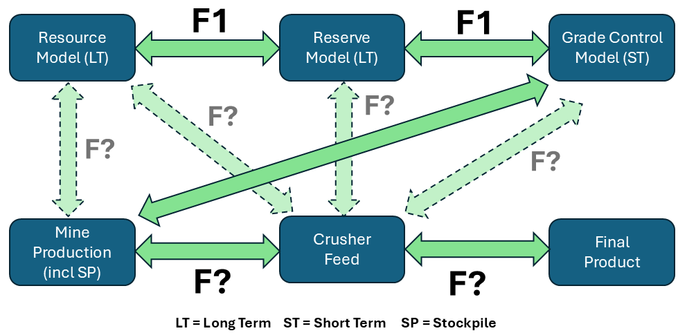
Mine reconciliation requires information such as initial predictions from exploration data and geological models, actual measurement: data from mining sources, such as blast holes, stockpile samples, or mill feed. As well it will need data on the final product being shipped off site. Do the metal quantities balance out throughout the mining operation?
Mine reconciliation tends to aggregate over longer time periods (monthly, quarterly or annually) due to short term impacts of material handling in stockpiles and plant circuits and the labour time needed to collect the input data.
Mine reconciliation ultimately attempts to assess how well the delivery of the final metal product relates to the initial resource model (i.e. what the project decision was originally based on)? It is also tool to evaluate the impact of any innovation implementation on the operation.
Reconciliation will help mine operators highlight issues and optimize extraction, manage costs, and ensure compliance with regulatory or investor expectations. Factors such as poor resource estimation, excessive dilution and ore loss, inaccurate sampling, etc. can cause discrepancies, making reconciliation an important part of any operation.
The reconciliation process is also used to derive Mine Call Factors. These factors are used to modify the forecasts from long range models, short range models, and grade control models to better represent the actual performance the operation will likely see. Large call factors suggest something is amiss in the “forecast to actual” progression. The first problem is to identify the causes. The list of the common sources of error can be lengthy. Then, once identified, the second problem is how to fix them.

Harry Parker initially suggested various reconciliation parametrics and labelled them F1, F2, F3. In a 2009 paper by Fouet titled “Standardising the Reconciliation Factors Required in Governance Reporting”, indicates that Rio Tinto had decided upon fifteen (15) different possible reconciliation correlations (see image below). Each one provides an insight on the efficiency of the operation in one way or another. I have seen modified versions of the reconciliation relationships, so it appears there may be no industry standard at this time. Fouet was asking about industry standardization in 2009 (an excellent paper to read by the way).

Mining Codes Getting Involved

It appears that the JORC Code may be recognizing the importance of reconciliation. In an August 2024 Exposure Draft JORC is suggesting the following text: “Where an Ore Reserve has been publicly reported for an operating mine, the results of both production reconciliation and any prior estimate comparison must also be included in the annual Mineral Resources and Ore Reserves statement. Refer to Clause 2.36. The relationships and variables being reconciled must be described in plain language or depicted graphically and must include reconciliations of both the Mineral Resources and Ore Reserves.”

Interestingly, it appears that NI43-101 has not yet jumped on the bandwagon about the importance of disclosing reconciliation results. However, it may just be a matter of time before it becomes one of their disclosure requirements.

If more regulatory focus will be put on mine reconciliation disclosure, then perhaps more industry standardization is warranted. This would help better define some of the terminology and “F factors” shown in the diagrams above to ensure consistency and help avoid each mine doing reconciliation in their own way.

Excel versus Cloud Based Reconciliation

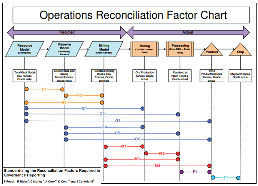
Each mine site may be unique with respect to; ore sources; terminology; ore types; mining methods; stockpiling philosophy; processing methods; technology availability; and personnel capability. So often the easiest approach for mine reconciliation is based on the Excel spreadsheet. (Reconciliation is generally not an easy undertaking).

Spreadsheets can be built site specific, based on an operation’s unique characteristics.

Spreadsheets are often built by a user for that user. They are tailored for the tailor. In my experience, typically the modeler is the only one comfortable with an Excel model’s logic, since all of us may think differently. Unfortunately, with the spreadsheet approach, it becomes more difficult to standardize an industry wide reconciliation process.

An alternate solution to spreadsheets is to use a cloud based standardized software package. Toronto based Minebright has one option, called Pit Info (see link for more info). There are a few other reconciliation software applications available. They tend to be cloud based, hence multiple people can have access to the input modules or output modules. (I would like to thank the Minebright people for steering me towards some of the technical papers on this subject).

The cloud based approach may help make reconciliation a group effort instead of a tightly controlled internal function. It may also help standardize reporting from a company’s multiple operations, reporting from the mining industry globally, or simply for consistent JORC reporting.

The downside to the cloud approach is the mine site teams must learn the software and tailor it to their operation. However, once that hurdle is passed, personnel changes become less onerous due to the model consistency. I have seen cases where a person doing the Excel reconciliation task has left their job, and hence forward the reconciliation effort came to a halt. The people remaining may be too busy or simply don’t want to have to figure out the Excel logic of someone else.

The other nice thing about a cloud software approach is that when improvements are rolled out, every user gets the same update. The “wisdom of crowds” will result in learnings and suggestions that will tend to improve the application functionality over time. There are a lot of smart people out there, and it would be nice to see them working together rather than individually, as the open source software community has demonstrated.

With AI, we also may get to the point where cloud based mine reconciliation platforms can use learnings from other projects, and help identify where the likely technical shortfalls are at a mine site and why production is not reconciling. Let’s ask AI do some of the thinking for us to get to the bottom of a problem.

Conclusion

Mine reconciliation is becoming more and more important, but it can be a forgotten aspect. Sometimes this is because it is difficult to do properly. However, that doesn’t mean it shouldn’t be attempted. The more one can learn about one’s operation, the more likely it can stay efficient, relevant, and in business. The more one knows whether technology improvements are making a difference, the more one may be willing to take on even more new technology.

Shifting some people (like me) away from Excel based solutions can be a challenge, but this is an area where it makes sense. Years ago, many engineers did mine production scheduling using Excel, but we have gradually moved away from that, thankfully. Reconciliation should maybe follow that path.

Disclaimer: Mining is a global business, and perhaps more progress is being made on reconciliation standardization than I am aware of sitting here in my Toronto office. Mine operations around the world are at the forefront of developing new systems. Perhaps we are seeing great things being done in the area of mine reconciliation, or maybe we are not. Please share your experiences if you’re comfortable doing that.

Note: You can sign up for the KJK mailing list to get notified when new blogs are posted. Follow me on Twitter at @KJKLtd for updates and other mining posts. The entire blog post library can be found at https://kuchling.com/library/

NPV a Disappointment? A Few Ways to Fix It

Date: April 5, 2024 Author: Ken Kuchling Comments: Leave a reply

So, you just completed your initial PEA cashflow model and the resulting NPV and IRR are a little disappointing. They are not what everyone was expecting. They don’t meet the ideal targets of an IRR greater than 30% and an NPV that is more than 2x the initial capital cost. The project could now be on life support in the eyes of some.

Now what to do? Its time to jump into NPV repair mode.

Hopefully this blog post isn’t too controversial but will lead to some discussion about how studies are done. Its based on observations I have made over the years as to what different studies will do to try to improve their economics.

The first thought typically is to lower (i.e. low ball) the capital and operating costs. We know that will certainly improve the economics. A risk with that is it might discredit the entire study if the costs are not in line with similar projects. Perhaps someone does a deep dive into the costing details or does some benchmarking against other projects. Also, advanced studies will develop more accurate costs, ultimately highlighting that the initial study was inaccurate and misleading. So overly optimistic, under-estimated costing is not a good approach.

What other things can help bump up the NPV? Let’s look at some of the ones I have seen, some of which I have applied in my work. I would expect (and hope) that some of these ideas will already have been adopted in the initial engineering and cashflow model.

Using the Time Value of Money

The discounting of cashflows in a cashflow model means that up-front revenues and costs have a bigger impact on the final economics than those far off in the future. This effect is amplified at higher discount rates.

Hence looking at ways to bring revenue forward or push costs backwards are typically the first options considered. Here are a few of the ways this will be done.

High Grading and Stockpiling: One can bring revenue forward by using a Low Grade Ore stockpiling strategy. Select an elevated cutoff grade to define High Grade Ore and send only that ore to the plant. The Low Grade Ore can be placed into a stockpile and processed gradually or all at once at the end of the mine life. One must mine more tonnes to undertake stockpiling and will eventually incur an ore rehandling cost. However, in my experience, the early revenue benefit from high grade normally outweighs the associated cost impacts.

Stockpiling Tramming: If using the stockpiling approach described above, many assume that all stockpile rehandling to the crusher will simply be done by tramming with a wheel loader. Having to re-load the ore into trucks will cost more than double the cost of tramming. So place the ore stockpiles close to the crusher to lower rehandling costs.

Milling Soft Ore: If the deposit has both an upper soft ore (oxide, saprolite) and a deeper hard ore, one can take advantage of the soft material and push more ore tonnage through the plant at start-up. This will increase the up-front revenue. It may also allow the cost deferral of some plant components that are only needed for processing the harder ore.

Defer Stripping Tonnages: Delaying some waste stripping costs from pre-production (Y-1) to Year 1 or Year 2 will help improve the NPV. However, care must be taken that increasing mining tonnages in Year 1 or 2 doesn’t trigger the purchase of additional loaders and trucks. The deferred tonnes need to be small enough not to trigger a fleet size increase or could negate the impact of the cost deferral.

Capitalize Waste Stripping: It may be possible to capitalize waste stripping for satellite pits and pit wall pushbacks to better align stripping costs with the timing of ore mining. Capitalizing waste stripping may result in lower short term taxable income since the entire expense is not immediately deducted. This can reduce tax liabilities and improve cash flow. Each situation may be unique.

Accelerate Depreciation: In some jurisdictions, tax laws permit accelerated depreciation rates. This will help to lower or eliminate taxable income in the early years. This boosts the after-tax cashflow in those years, bumping up the NPV. If accelerated depreciation is the case, enhancing revenue (by high grading) at the same time, gives an even bigger nudge to the NPV. Maximize the revenue during tax free periods.

Apply Tax Losses: On some projects there are historical corporate tax loss carry-overs. These losses allow one to offset future taxes payable in the early years. This help bump up the initial after-tax cashflows.

Leasing of Equipment: One can look at equipment leasing to defer some of the initial capital costs. Leasing will distribute the purchase cost over several years (typically 60 months). Although the lease interest will increase the total cost of the machine, the capital cost deferral likely results in an NPV benefit.

Use Contract Mining: To avoid the entire cost of purchasing major mining equipment, many will look to contract mining. In studies, sometimes contract mining costs are estimated or they can be derived from budgetary contractor quotes. At an early stage these contractor quotes might be quite “favorable” as the contractor tries to stay in the good books of the mining company. Contract mining will greatly reduce the mining equipment capital cost and can help the NPV, even if the unit mining costs may be slightly higher with a contractor.

Using Other Cashflow Tweaks

There are other tweaks that one can make to the cashflow model. Sometimes several of the small ones, when compounded together, will result in a significant impact. Here are some of the other cashflow model adjustments that I have seen.

Increase Metal Prices: Normally when selecting metal prices for the cashflow model one looks at; trailing averages; analyst consensus forecasts; marketing study forecasts; and prices being used in other current studies. It is usually simple to defend whatever price you wish to use. In a rising price environment, one can see what other recent studies have used and escalate those prices by 5%-10%. That likely won’t be viewed as unreasonable. After all, someone has to be the trailblazer in raising modelling metal prices.

Improve metal recoveries: At an early study stage, one may have limited number of metallurgical tests upon which to base the process recoveries. I have seen some bump up the recoveries slightly and add the statement “Further metallurgical testing, grind size optimization, and reagent optimization should improve the recovery above those shown by the current test work”. This can gain a bit of revenue at no extra cost.

Optimistic Dilution: It can be very difficult to predict ore mining dilution at an early stage. Two different engineers looking at he same mining method, may come up with different dilution assumptions. Hence one may have the opportunity to select an optimistic dilution. Lower dilution will increase the head grade to the mill and hence increase the revenue at no extra cost. Even a modest reduction in dilution will play its role in nudging up the NPV.

Reduction in Working Capital: Some cashflow models do not include the cost for working capital, while others will include it. Working capital is the money needed on hand to pay the monthly operating cost in Year 1 before payable revenue is generated. If difficulties arise in achieving commercial production, one wishes to have more working capital on hand. Working capital typical is 2-4 months of operating cost. To bump up NPV, some will use the lower range of 2 months working capital. Some will just omit working capital entirely. Take a look at the working capital needs and decide what is reasonable.

Buy the Royalty: Some projects may have the option for a company to buy out the royalty from the royalty holder. Although doing this may result in an upfront cost, the payable royalty saving may offset that up-front buy-out cost. At high metal prices, the royalty saving could be significant.

Reclamation Cost Equals Salvage Value: At the end of the mine life, the final closure and reclamation cost will be in the tens of millions of dollars. Although this cost is heavily discounted back to the start of the cashflow model, I have seen cases where it is assumed that salvage value of the mine and plant equipment is sufficient to pay the entire closure cost. I don’t know how realistic this is, but I have seen that assumption used.

Lower The Discount Rate: A few years ago, it seems the benchmark discount rate was 5% used in most studies. In 2024, the cost of capital has gone up. Hence many studies seem to be using 8%-10% as their base case. A project at the PEA stage today isn’t going to be built for a few years. Some can argue that interest rates will likely be lower in a few years, and so using 5% discount rate today is still reasonable. Conversely some will maintain that is is best to use what others are using so that current projects are all comparable.

Conclusion

Don’t let a disappointing NPV get you down. There may be a few ways to boost the NPV by applying some common practices. However, if after applying all of these adjustments, the NPV still isn’t great, something bigger may be required. That could be an entire project scope re-think.

Or go drill for more ore higher grade ore.

Or low-ball the cost estimates (just kidding).

I have heard that if the project requires fancy tax manipulation to make it work, then it isn’t a good project to begin with. If taxes are critical, the economics may be too marginal.

Note: You can sign up for the KJK mailing list to get notified when new blogs are posted. Follow me on Twitter at @KJKLtd for updates and other mining posts. The entire blog post library can be found at https://kuchling.com/library/

The Anatomy of 43-101 Chapter 16 – Mining (Part 2)

Date: March 22, 2024 Author: Ken Kuchling Comments: Leave a reply

Part 2 of this blog post will focus on the remaining engineering work to finish Chapter 16 of the Technical Report. We only wrote about half of it in Part 1. The mining engineer can generally handle the rest of these tasks without requiring a lot of external input. You can read Part 1 at this link “The Anatomy of 43-101 Chapter 16 – Mining (Part 1)”.

The pit design and phases were completed at the end of Part 1, and we can move on to scheduling.

4. Production Scheduling

Once the pit design is complete, everyone will be calling for the production schedule as soon as possible. Others on the team are waiting for it. The tailings engineers need the production schedule for the tailings stage design. The process engineers need the scheduled head grades to finalize sizing the plant components. The client wants the schedule to plug into their internal cashflow model for a quick peek at the economics.

However, before the mine engineer can start scheduling, the dilution approach needs to be selected. Dilution is waste that is mixed in with ore during mining. A high amount of dilution can dramatically lower the processed head grades. There may be a desire to “low ball” the dilution to make the grades look better, but the engineer should base the dilution on what they would expect to see.

Two dilution approaches are common. One can either construct a diluted block model; or one can apply dilution afterwards in the production schedule. I have used both approaches at different times.

The production schedule must be on a diluted basis, since that represents what the processing plant will actually see.

Generally, two different production schedules must be created: (i) a Mining schedule, and (ii) a Processing schedule. In some instances, they may be one and the same schedule. However, if any ore stockpiling is done, then the Mining schedule will be separate from the Processing schedule.

The Mining schedule shows ore going directly to the plant and ore going into the stockpiles. The Processing schedule will show ore delivered directly from the mine and ore reclaimed from stockpiles. Building stockpiles and pulling ore from stockpiles are two independent activities.

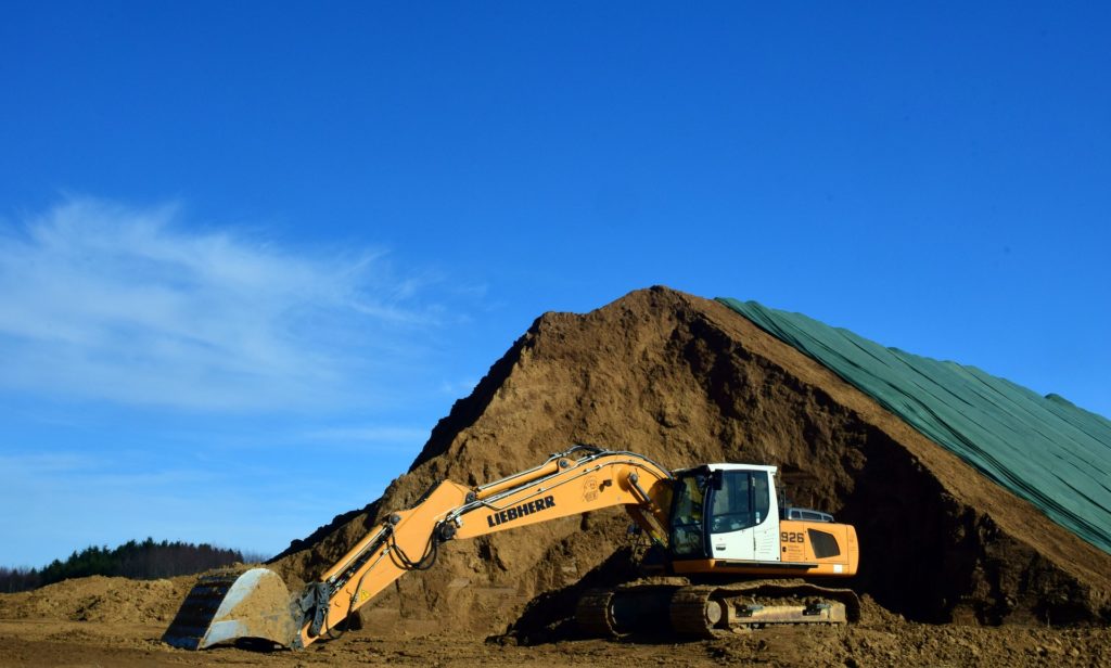
Sometimes lower grade stockpiles are built up by the mine each year but only processed at the end of the mine life. Periodically the ore mining rate may exceed the processing rate and other times it may be less. This is where the stockpile provides its service, smoothing the ore delivery to the plant.

Scheduling can be done with variable time periods. Perhaps the schedule is generated using monthly time periods, or quarters, or years.

The 43-101 report will normally show the annual production schedule, but that does not mean it was generated that way. I prefer to use short time periods (monthly or quarterly) for the entire mine life, to ensure ore is always available to feed the plant. A 10 year mine life would result in 120 monthly time periods, so output spreadsheets can get large.

Scheduling can be done manually (in Excel) or by using commercial software, like Datamine’s NPVS. The commercial software is better in that it allows one to run different scenarios more quickly, and it does a lot of the thinking for the engineer. It also does a good job of stockpile tracking. It also decides when it is necessary to transition to mining in satellite pits.

Once the schedules are finalized, they are normally reviewed by the client for approval. The strip ratio and ore grade profile by date are of interest. One may then be asked to look to at different stockpiling approaches to see if an NPV (i.e. head grade) improvement is possible.

One can stockpile lower grade ore and feed the plant with better grade by mining at a higher rate with more equipment. One might need to examine iterative schedules of that type.

Sometimes one must take two steps backwards and re-design some of the initial pit phases to reduce waste stripping or improve grades. Then one would run the schedules again until getting one that satisfies everyone.

Now that the schedule is complete, we can write up the Chapter 16 text up to page 15. We’re getting closer to the end.

5. Site Layout Design

With the pit tonnages and mining sequence from the schedule, the mine engineers can start to look at the site layout (waste dumps and haul roads). Normally the tailings engineers will be responsible for the tailings layout. However, if there is no tailings engineer on the PEA team, the mining engineer may look after this too.

First there is a need for a waste balance. This defines how much mined overburden or waste rock will be needed to build haulroads, laydown pads, and tailings dams. Then the remaining waste volume must be placed into waste dumps.

Hopefully the tailings engineers have finished their tailings dam construction sequence by this time to provide their rockfill needs (although unlikely if you only gave them the production schedule two days ago).

The geotechnical engineers will provide the waste dump design criteria; for example, 3:1 overall side slope using 15m high dump lifts. Ideally it is nice to have soil and foundation information beneath the waste dump sites, but at PEA stage most often this isn’t available. The dump locations are only being defined now.

The mining engineers will size the various waste dumps to their required capacity. Then they can lay out the mine haulroads from the pit ramps exits to the ore crusher, the ore stockpiles, and to each waste dump.

That’s it for the site layout input. Add another 2 pages to Chapter 16. Now the mining engineers can look at the mining equipment fleet.

6. Fleet Sizing and Mining Manpower

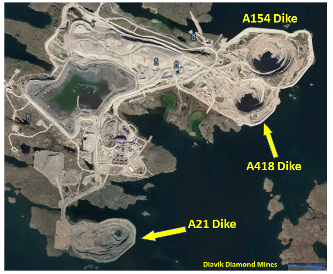
The last task for the mine engineer in Chapter 16 is estimating the open pit equipment fleet and manpower needs. The capital and operating costs for the mining operation will also be calculated as part of this work, but the costs are only presented in Chapter 21.

The primary pieces of equipment are the haul trucks. They can range in size from 30 tonnes to 350 tonnes and anywhere in between.

Typically, the larger the equipment is, the lower the unit cost ($/t), especially in jurisdictions where labor costs are high. One doesn’t want a mine fleet with only 5 trucks nor one with 50 trucks. So where is the happy medium?

Once the schedule and site layout are complete, the mine engineers can run the truck haul cycles, in minutes. They need to estimate the time to drive from the pit face, up the ramp, to the waste dump, to the ore crusher, and return back into the mine. Cycle times determine the truck productivity, in tonnes per hour per truck and include the time to load the truck. Some destinations may have long cycle times (to a far off crusher) while others may be quick (to an adjacent waste dump).

The cycle time must be calculated for each material type going to each destination. As the pit deepens, the cycle times increase.

Very simplistically, if a 100 tonne truck has a 20 minute cycle time, it can do three cycles in an hour (300 tph). If one has to mine 10 million tonnes of ore per year, then that would require 33,300 truck hours. If a single truck provides 6500 operating hours per year, that activity would require a fleet of 5 trucks. The same calculation goes for waste.

The total trucking hours will vary year to year as waste stripping tonnages change or haul cycle times increase in deeper pits. The required truck fleet may vary year to year. Keeping haul distance short and haul cycles quick is the key to a lower cost mine.

The mine engineers undertake the productivity calculations for loading equipment to estimate annual operating hours, and the required shovel / loader fleet size.

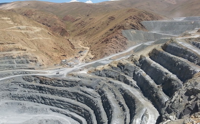
The support equipment needs (dozers, graders, pickups, mechanics trucks, etc.) are typically fixed. For example, 2 graders per year regardless if the annual tonnages mined fluctuate.

The support equipment needs are normally based on the mining engineer’s experience. Hence the benefit of actually working at a mine at some point in your career.

Blasting includes both the blasthole drilling activity and hole charging. The mining engineer estimates drill productivity and specifications based on the bench height, the expected rock mass quality, and the power factor (kg/t) need to properly demolish the rock.

Finally, the mine operation manpower is estimated based on all the equipment operating hours as well as the fixed number of personnel to support and supervise the mine.

This essentially concludes the mining information presented in Chapter 16 of a typical 43-101 open pit report.

Conclusion

These two blog posts hopefully give an overview of some of the things that mining engineers do as part of their jobs. Hopefully the posts also shed light on the amount of work that goes into Chapter 16 of a 43-101 report. While that chapter may not seem that long compared to some of the others, a lot of the effort is behind the scenes.

Some will say PEA’s are not very accurate documents that should be taken with a grain of salt. One should understand that engineers are working with a limited amount of information at this early stage while forming the concept for the proposed operation.

The subsequent study stages are where more accurate costs are expected and can be demanded.

I don’t know if this overview makes one want to sign up to be a mining engineer or learn to code instead. None of this is rocket science; it just requires practical thinking.

If young people want to get into mining, but not sure into which aspect, I suggest go read through a 43-101 report. There are sections describing exploration, resource modelling, mine engineering, metallurgy, geotechnical engineering, environmental, and financial modelling. Its all in one document. See if any of these areas are of interest to you. Universities should use 43-101 reports as part of their mining engineering curriculum.

Note: You can sign up for the KJK mailing list to get notified when new blogs are posted. Follow me on Twitter at @KJKLtd for updates and other mining posts. The entire blog post library can be found at https://kuchling.com/library/

Mine Builders vs Mine Vendors

Date: October 15, 2023 Author: Ken Kuchling Comments: Leave a reply

Normally when Major or Intermediate miners advance their projects through the study stages, they usually have the intent to build the mine at some time. Sometimes they may decide to sell the project if it no longer fits in their corporate vision or if they desperately need some cash. However, selling the project was likely not their initial intent.

On the other hand, Junior miners tend to follow one of two paths. They are either on (a) the Mine Builder path, or (b) the Mine Vendor path (i.e. sell the project). In this article, I will present some examples of companies on each path. There will also be some discussion on whether the engineers undertaking the early stage studies (e.g., PEA’s) should be considering the path being followed.

The Mine Builder Path

The Mine Builder generally follows a systematic approach, as sketched out in the image below. The project advances from drilling to Mineral Resource Estimate (MRE), scoping study (PEA), then through the Pre-Feasibility Study (PFS) and/or Feasibility Study (FS) stages. Environmental permitting is normally proceeding in conjunction with the engineering. Once the FS is complete, the next hurdles for the Mine Builder are financing and construction. The path is fairly orderly.

The amount of the exploration drilling is only needed to define an economic resource to the Measured and Indicated classifications. There is no requirement to delineate the mineral resource on the entire property since there will be time to do that during production. Demonstrating an economic resource, with some upside potential, is often sufficient for the Mine Builder.

Three examples of companies on the Builder path are shown below; Orla Camino Rojo gold project (in operation), SilverCrest Las Chispas gold project (in operation), and Nexgen Rook uranium project (financing stage). Although the duration of each timeline is different due to different project complexities, the development paths are consistent. Most junior miners would not consider themselves on the Builder path.

The Mine Vendor Path

Mine Vendor type organizations have the primary goal of selling their project. These companies may consist of management teams that don’t have the desire, comfort, or capability to put a mine into production. For example, this is often the case with companies founded by exploration geologists, whereby their plan is to explore, grow, and sell all (or part) of the project. In other cases the Junior miner realizes their project is large with a high capital cost. That capital cost is beyond the financial capability of the company. Hence a deep-pocket partner is required or an outright sale is preferred.

The Mine Vendors tend to follow a different development path than the Mine Builders. They don’t have the same long term objectives. Vendors want out at some point.

The Vendor path can be more irregular, with multiple studies undertaken at different levels of detail, sometimes stepping back to lower level of studies as more information is acquired. Their object is to make the project look good to potential buyers, and look better than their junior miner competitors also for sale. Often this ongoing project improvement process is termed “de-risking”.

Not only must the Vendors demonstrate an economic resource, they must demonstrate a highly valuable resource to maximize the acquisition price for the shareholders. They will try to do this through multiple drill campaigns followed by multiple studies, each one looking better than the prior one.

Sometimes you will see a management team indicate that, if the project isn’t sold, they are going to put it into production themselves. This may be true in some cases, or simply part of the negotiating game to try to maximize the acquisition price.

Two quick examples of companies on the Vendor path are shown below: Western Copper Casino project and Seabridge KSM project. The durations of these development timelines are extensive and expensive, while waiting for an interested buyer. During these periods, the companies may continue to spend money de-risk the project further. The hope is that the company can eventually make the project attractive or that changing market conditions will make it attractive for them. Unfortunately, there is always the possibility that no buyer will ever come along.

Engineer’s Perspective

One question is whether the independent geologists and engineers working on the advanced studies should be aware of the path the company is following. Is the company a Builder or a Vendor?

Some may feel that the technical work should be independent of the path being followed. Based on my experience as both an owner’s representative and independent study QP, I have a somewhat different opinion. The technical work should be tailored to the intended path.

The Engineer on the Mine Builder Path:

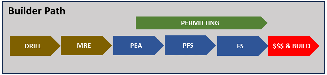
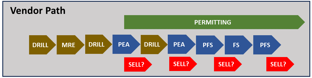
If an engineer understands that a Mine Builder’s project will move from PEA to PFS to FS in rapid succession, then there is more incentive to ensure each study is somewhat integrated.

For example, a PEA will use Inferred resources in the economics. However, if the project will advance to the PFS stage, where Inferred cannot be used, then it is important for the PEA to understand the role that Inferred plays in the economics. How much drilling will be needed to upgrade Inferred resource to Indicated for the PFS, if needed at all?

Typically, capital costs tend to increase as advancing studies get more accurate due to greater levels of engineering. A Builder wants to avoid large cost increases when moving from PEA to PFS to FS. Therefore, when costing at the PEA stage, one may wish to increase contingency or use conservative design assumptions. After all, one is not trying to sell or promote the project internally, but rather move it towards production.

There is no value to the Mine Builder by fooling themselves with low-balled cost estimates. (Although some may argue there is still a desire to low ball costs to get management to approve the project). Conversely Mine Vendors do have some incentive to low ball the costs.

Perhaps some of the recent project capital cost over-runs we have seen is that the Vendor mentality was used at the PEA stage to optimistically set the capital cost baseline. Subsequent studies were then forced to conform to that initial baseline. Ultimately construction will be the arbiter on the true project cost. Hence there is no real value in underestimating costs, ultimately making management appear incompetent if costs do over-run.

The Mine Builder will also be advancing environmental permitting simultaneously with their advanced studies. Hence at the early stage (PEA) it is important to properly define the site layout, processing method, production rate, facility locations, etc. since they all feed into the permitting documents.

Changing significant design details in the future will set back the permitting and construction timelines. Hence, for the Mine Builder, the engineers should focus on getting the design criteria mostly correct at the PEA stage. For the Mine Vendor, this is not as important since multiple studies are being planned for in the future anyway.

The Engineer on the Mine Vendor Path:

The objective of the Mine Vendor is to make the project attractive to potential buyers. There is less urgency in fast tracking detailed engineering and permitting.

It is not uncommon to see multiple drilling programs, followed my multiple studies of scenarios with different size, production rate, and layout. The degree of engineering conservativeness in design and costing is less critical since future studies may be on substantially different sized projects.

The role that the Inferred resource plays in the economics is also less important at this time, since a lot more drilling may be coming. The Vendor’s objective tends to be on maximizing resource size not necessarily optimizing resource classification.

While the Mine Vendor may also be advancing environmental permitting as another way to de-risk the project, the project design may still be in flux as the resource size changes. Major modifications to the plan may cause permitting to stop and re-start, leading to an extended project timeline and wasted money.

There is also risk in starting the permitting with a project definition that isn’t of economic interest to future buyers. Sometimes the Vendor may be making regulatory commitments that constrain the operating flexibility of future mine operators. Its easy to commit to things when you aren’t the one having to live up to them.

The Mine Vendor will also de-risk the project by moving from PEA to PFS and even to FS. The caution with completing a FS is that it is a costly study and essentially brings one to the end of the study line. What does the company do next if there is still no buyer?

Feasibility studies also have a shelf life, with the cost estimates and economics becoming inaccurate after a few years. Some companies may re-examine the project, re-frame it, and jump back to the PEA or PFS stages. There can be an on-going study loop, requiring continued funding with no guarantee of a sale in sight. Often feasibility studies have the dual role of trying to boost the share price and market cap, as well as frame the project for potential buyers.

Conclusion

As an engineer, it is helpful to understand the objectives of the project owner and then tailor the technical studies to meet those objectives. This does not mean low balling costs to make the study a promotional tool. It means focusing on what is important. It means recognizing the path, and what doesn’t need to be engineered in detail at this time. This may save the client time, money, and improve credibility in the long run.

In many cases, the precise size of the deposit is less important than understanding the site, access, water supply, local community issues, the environmentally acceptable location for dumps and tailings, etc.. It can be more important to focus on these issues rather than having a detailed mine plan with multiple pit phases that immediately becomes obsolete in a few months after the next drilling campaign.

Potential buyers will have their own technical team that will develop their own opinions on what the project should be and what it should cost. Just because a Mine Vendor has a feasibility study in hand, doesn’t mean a potential buyer will believe it.

This post is just a brief discussion of mining project timelines. For those interested, there a few additional project timelines for curiosity purposes. Each path is unique because no two mining projects are the same. You can find these examples at this link “Mining Project Timelines”.

Let me know about other interesting projects that have interesting paths to learn from. I can add them to the list.

Note: You can sign up for the KJK mailing list to get notified when new blogs are posted. Follow me on Twitter at @KJKLtd for updates and other mining posts. The entire blog post library can be found at https://kuchling.com/library/

Grade-Tonnage Curves – Worthy of a Good Look

Date: July 16, 2023 Author: Ken Kuchling Comments: Leave a reply

Most of us have seen the typical “grade-tonnage” table or graph, showing ore tonnes and grade at varying cutoff grades. It is usually part of every 43-101 technical report in Section 14. We may glance at it quickly and then move on to more exciting chapters. Section 14 (Mineral Resources) can be a very complex chapter to read with statistics, geostatistics, and mathematical formulae. However the grade-tonnage curve aspect isn’t complicated at all.

The next time you see the grade-tonnage relationship, I suggest taking a few seconds to study it a bit further. There might be some interesting things in there.

Typical Grade-Tonnage Information

Typically, one will see grade-tonnage data in 43-101 Technical Reports towards the back of Section 14 "Mineral Resources". The information is normally presented in either of two ways; (i) a grade-tonnage table or (ii) a grade tonnage graph. Examples of each are shown below. The grade tonnage graph typically has the cutoff grade along the bottom x-axis and the two separate y-axes representing the ore tonnes above cutoff and the average ore grade above cutoff.

Rarely do you see both the table and curve in the report, although ideally one would want to see both. Given the option, I would prefer to see the graph more than the table of numbers. The trend of the grade-tonnage information is just as important as the values, maybe even a bit more important. Unfortunately, a data table by itself doesn’t illustrate trends very well.

Useful Grade-Tonnage Curve Information

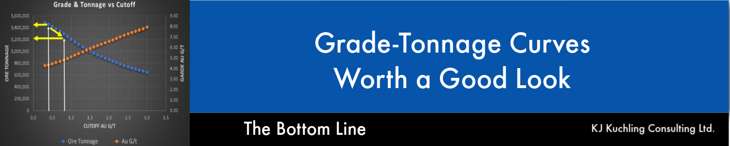
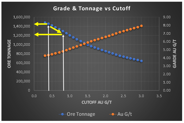
When I am undertaking a due diligence review or working on a study, very early on I like to have a look at the grade-tonnage information. This could be for the entire deposit resource, within a resource constraining shell, or in the pit design.

The grade-tonnage information gives an understanding of how future economics or technical issues may impact on the mineable tonnage.

An example of a typical grade-tonnage curve is shown here.

The cutoff grade along the x-axis will be impacted by changes in metal price or operating cost. The cutoff grade will increase if metal prices decrease or if operating costs increase.

The question is how sensitive is the mineable tonnage to these economic factors. The slope of the tonnage and grade curves will help answer this question.

In the example shown, the tonnage curve (blue dots) is fairly linear, meaning the ore tonnage steadily decreases with increasing cut-off grade. That is expected and is reasonable.

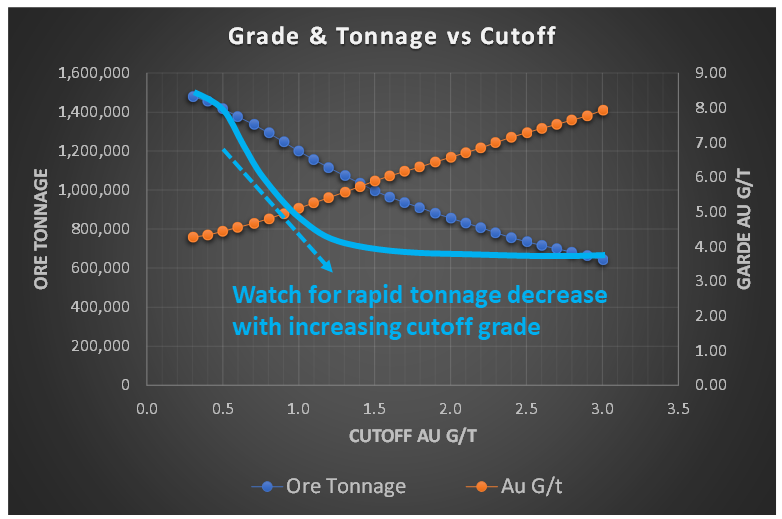
However, if the tonnage curve profile resembled the light blue line in this image, with a concave shape, the ore tonnage is decreasing rapidly with increasing cutoff grade. This is generally not a favorable situation.

It indicates that a significant portion of the tonnage has a grade close to the cutoff grade. If that’s the situation, the calculation of the cutoff and the inputs used to generate it are important and worthy of scrutiny. Are they reasonable? Over the long term, is the cutoff grade more likely to increase or decrease?

The same logic can be used with the ore grade curve in the graph. As shown in this example, the ore grade increases steadily as the cutoff is raised. This is because lower grade ore is being shifted from ore to waste, and hence the remaining ore has better quality. If the cutoff is raised from 0.4 g/t to 0.5 g/t, then some material with a grade of about 0.45 g/t is moved from ore to waste.

I also like to compare the ratio of the average grade to the cutoff grade. Its nice to see a ratio of 4:1 to 5:1 to ensure the overall average grade isn’t close to the cutoff. In this example, the cutoff grade is 0.5 g/t and the average grade is 4.5 g/t, a ratio of 9:1.

The tonnage curve and grade curve provide information on the nature of the mineral resource. Study them both.

Reporting Waste Within a Shell

One complaint I have about reporting mineral resources inside a resource constraining shell is the lack of strip ratio information. This applies whether disclosing a single mineral resource estimate or variable grade-tonnage data.

In my view, the strip ratio is even more important to be aware of when looking at grade tonnage data.

The strip ratio within a shell will climb as an increasing cutoff grade results in a decreasing ore tonnage. Sometimes the strip ratio will increase exponentially. The corresponding amount of waste remaining in that pit shell increases, hence the ratio of the two (i.e. strip ratio) can escalate rapidly.

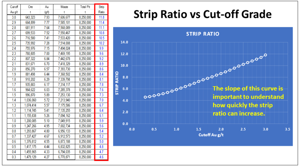
Regarding mineral resources, one should be required to disclose the waste tonnage and strip ratio when reporting resources inside a constraining shell. The constraining shell and cutoff grade are both based on defined economic factors such as unit mining costs, processing cost, process recoveries, and metal prices. With respect to the mining cost component, the strip ratio is a key aspect of the total mining cost, yet it normally isn’t disclosed.

Its common to see mention that the mining cost is (say) $2.50/t, but if the strip ratio is 10:1, that equates to an effective mining cost of $27.50 per tonne of ore. That’s an important cost to know, especially if one is pushing a pit shell deep to maximum the mineral resource tonnage.

Each mineral deposit resource model can behave differently. Hence, in my view, the waste tonnage should be included when reporting mineral resource tonnages (or presenting grade-tonnage data) within a constraining shell. This waste tonnage or strip ratio can be in the footnotes to the mineral resource summary table.

Spider Diagram Downsides

In 43-101 technical reports, the financial Chapter 22 normally presents the project sensitivities expressed in a spider diagram or a table format.

In a previous blog post I had discussed the flaws in the spider diagram approach. That article link is at “Cashflow Sensitivity Analyses – Be Careful”. The grade-tonnage curve helps explain why that is.

In the spider diagrams, we typically see sensitivities related to +/- 20% on metal prices and operating costs. If either of these factors change, then in reality the cutoff grade would change.

If the metal price decreases by -20%, or the operating cost climbs by +20%, the cutoff grade must increase. This adjustment is normally not made in the sensitivity analysis because it requires a lot of re-work.

Elevating the cutoff grade would shift the pit ore tonnage towards the right on the grade-tonnage curve, showing a decrease in mineable tonnes. However, in the spider diagram logic, the assumption is that production schedule in the cashflow model is unchanged and simply the metal prices or operating costs are adjusted. Therefore, the spider diagram can be a misleading representation of the downside risk, showing a more positive situation than in reality.

Conclusion

The grade-tonnage information is always presented in technical reports. It examines the sensitivity of the orebody size to changes in cutoff grade. The next time you see grade-tonnage data, don’t skip over it. Take a minute to study it further to see what can be learned.

Note: You can sign up for the KJK mailing list to get notified when new blogs are posted. Follow me on Twitter at @KJKLtd for updates and other mining posts. The entire blog post library can be found at https://kuchling.com/library/

Mining Under Lakes – Part 2: Design Issues

Date: June 11, 2023 Author: Ken Kuchling Comments: 3 Replies

This is Part 2 of a blog post related to open pit mining within bodies of water. Part 1 can be found at this link “Mining Under Lakes – Part 1“, which provides a few examples where this has been done successfully. Part 2 focuses on some of the social and technical issues the need to be considered when faced with the challenge of open pit mining within a water body.

The primary question to be answered is whether one can mine safely and economically without creating significant impacts on the environment.

The answer to this question will depend on the project location and the design of the water retaining structure.

I have worked on several projects where dike structures were built. I have also undertaken due diligence reviews of projects where dikes would be required. Most recently I have participated in some scoping level studies where mining within a lake or very close to a river were part of the plan.

In some instances, the entire orebody is located in the lakebed. In others, the orebody is mainly on land but extends out into the water. Each situation will be unique. In northern Canada, given the number of lakes present, it would be surprising if a new mining project isn’t close to a river or lake somewhere.

Dike concepts consider many factors

Different mining projects may use different styles of dikes, depending on their site conditions. Some dikes may incorporate sheet piling walls, slurry cutoff walls, low permeability fill cores, or soil grouting. There are multiple options available, and one must choose the one best suited for the site.

The following is list of some of the key factors and issues that should be examined.

ESG Issues

One’s primary focus should be on whether building a dike would be socially and environmentally acceptable. If it is not, then there is no point in undertaking detailed geotechnical site investigations and engineering design. One must have the “social license” to proceed down this path.

Water Body Importance: Is there a public use of the water body? It could be a fresh water source for consumption, used for agricultural or fishery purposes, or used as a navigable waterway, etc. Would the presence of the dike impact on any of these uses? Does the water body have any historical or traditional significance that would prevent mining within it?

Lake Turbidity: Dike construction will need to be done through the water column. Works such as dredging or dumping rock fill will create sediment plumes that can extend far beyond the dike. Is the area particularly sensitive to such turbidity disturbances, is there water current flow to carry away sediments?

At Diavik, a floating sediment curtain surrounding the dike construction area was largely able to contain the sediment plume in the lake.

Regional Flow Regime: Will the dike be affecting the regional surface water flow patterns? If the dike is blocking a lake outflow point, can the natural flow regime be maintained during both wet and dry periods?

Location Issues

If there are no ESG issues preventing the use of a dike, the next item to address is the ideal location for it.

Water depth: normally as the dike moves further away from land, both the water depth and dike length will increase. The water depth at the deepest points along the dike are a concern due to the hydraulic head differential created once the interior water pool is pumped out. The seepage barrier must be able to withstand that pressure differential, without leaking or eroding. A low height dike in shallow water may be able to use a simpler seepage cutoff system than a dike in deep water.

Islands: Are there any islands located along the dike path that can be used to shorten the construction length and reduce the fill volumes? Is there a dike alignment path that can follow shallower water zones?

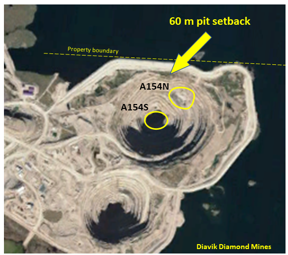
Pit wall setback: Given the size and depth of the open pit, how far must the dike be from the pit crest? Its nice to have 200 metre setback distance, but that may push the dike out into deeper water.

If the dike is too close to the pit, then pit slope failures or stress relaxation may result in fracture opening and increase the risk of seepage flows or catastrophic flooding. The pit wall rock mass quality will be the key determining factor in the setback distance.

Maximizing ore recovery: If the ore zone extends further out into the lake, maximizing ore recovery may require using a steep pit wall along the outer sections of the pit. This may require positioning haulroads with switchbacks along other sides of the pit rather than using a conventional spiral ramp layout.

At Diavik (see image), the A154 north open pit wall was pushed to about 60 metres of the dike to access as much of the A154N kimberlite ore as possible. Haulroads were kept to the south side of the pit.

It may be possible to recover even more ore by pushing out the dike even further. However, this may result in a larger and costlier dike or even require a different style of dike. There will be a tradeoff between how much additional ore is recovered versus the additional cost to achieve that. There will be a happy medium between what makes both technical sense and economic sense.

Design Issues

Once the approximate location of the dike has been identified, the next step is to examine the design of the dike itself. Most of the issues to be considered relate to the geotechnical site conditions.

Lakebed foundation sediments: What does the lakebed consist of with respect to soft sediments? Soft sediments can cause dike settlement and cracking, or mud-waving of fill material.

Will the soft sediments need to be dredged prior to construction, and if so, where do you dispose of this dredge slurry, and what impact will dredging have on the lake turbidity?

Lakebed foundation gravels: Are there any foundation gravel layers that can act as seepage conduits beneath the dike? If so, will these need to be sub-excavated, or grouted, or cut off with some type of barrier wall? Sonic drilling, rather than core drilling, is a better way to identify the presence of open gravel beds.

Upper bedrock fracturing: Is the upper bedrock highly fractured, thereby creating leakage paths? If so, then rock grouting may be required all along the dike path to seal off these fractures.

Major faults: Are there any major faults or regional structures that could connect the open pit with the lake, acting as a source of large water inflow?. At Diavik, we attempted to characterize such structures with geotechnical drilling before construction. Upon review, I understand there was one such structure not identified, which did result in higher pit inflows until it was eventually grouted off.

Water level fluctuations: In a lake or river one may see seasonal water level fluctuations as well as storm event fluctuations. The height of the dike above the maximum water level (i.e. freeboard) must be considered when sizing the dike.

Ice scouring: In a lake or river that freezes over, ice loads can be an important consideration. During spring breakup as the ice melts, large sheets of ice can be pushed around and may scour or damage the crest of the dike. The dike must be robust enough to withstand these forces.

Construction materials available on site: Is there an abundance of competent rock for dike fill? Is there any low permeability glacial till or clay that can be used in dike construction? If these materials are available on site, the dike design may be able to incorporate them. If such materials are not available, then a alternate dike design may be more appropriate, albeit at a cost.

Conclusion

Each mine site is different, and that is what makes mining into water bodies a unique challenge. However many mine operators have done this successfully using various approaches to tackle the challenge.

Even at the exploration stage, while you are still core drilling the orebody through the ice, you can start to collect some of this information to help figure it all out.

The bottom line is that while mining into a water body is not a preferred situation, it doesn’t mean the project is dead in the water. It will add capital cost and environmental permitting complexity, but there are proven ways to address it.

On the opposite side, I have also seen situations where a dike solution was not feasible, so ultimately there are no guarantees that engineers can successfully address every situation. Lets hope your project isn’t one of them.

There could be a 3rd part to this post that discusses issues associated with underground mining beneath bodies of water; however that is not my area of expertise. I would be more than happy to collaborate on a article with someone willing to share their knowledge and experience on that subject.

Note: You can sign up for the KJK mailing list to get notified when new blogs are posted. Follow me on Twitter at @KJKLtd for updates and other mining posts. The entire blog post library can be found at https://kuchling.com/library/

NPV One – Cashflow Modelling Without Excel

Date: May 21, 2023 Author: Ken Kuchling Comments: Leave a reply

From time to time, I encounter interesting software applications related to the mining industry. I recently became aware of NPV One, an Australian based, cloud hosted application used to calculate mineral project economics. Their website is https://npvone.com/npvone/

NPV One is targeting to replace the typical Excel based cashflow model with an online cloud model. It reminds me of personal income tax software, where one simply inputs the income and expense information, and then the software takes over doing all the calculations and outputting the result.

NPV One may be well suited for those not comfortable with Excel modelling, or not comfortable building Excel logic for depreciation, income tax, or financing calculations. These calculations are already built in the NPV One application.

I had a quick review of NPV One, being given free access to test it out. I spent a bit of time looking at the input menus and outputs, but by no means am I proficient in the software after this short review.

Like everything, I saw some very good aspects and some possible limitations. However, my observations may be a bit skewed since I do a lot of Excel modelling and have a strong comfort level with it. Nevertheless, Excel cashflow modelling has its own pro’s and con’s, some of which have been irritants for years.

NPV One – Pros and Cons

Pros

NPV One develops financial models that are in a standardized format. Models will be very similar to one another regardless of who creates it. We are familiar with Excel “artists” that have their own modelling style that can make sharing working models difficult. NPV One might be a good standard solution for large collaborative teams looking at multiple projects while working in multiple offices.
NPV One, I have been assured, is error free. A drawback with Excel modelling is the possibility of formula errors in a model, either during the initial model build or by a collaborator overwriting a cell on purpose (or inadvertently).
With NPV One, a user doesn’t need to be an Excel or tax modelling expert to run an economic analysis since it handles all the calculations internally.
NPV One allows the uploading of large input data sets; for example life-of-mine production schedules with multiple ore grades per year. This means technical teams can still generate their output (production schedules, annual cost summaries, etc.) in Excel. They can then simply import the relevant rows of data into NPV One using user-created templates in CSV format.
As NPV One evolves over time with more client input, functionality and usability may improve as new features are added or modified.

Cons

Like anything, nothing is perfect and NPV may have a few issues for me.

Since I live and breathe with Excel, working with an input-based model can be uncomfortable and take time to get accustomed to. Unlike Excel, in NPV One, one cannot see the entire model at once and scroll down a specific year to see production, processing, revenue, costs, and cashflow. With NPV jump to. If you’re not an avid Excel user, this issue may not be a big deal.
In Excel one can see the individual formulas as to how a value is being calculated. Excel allows one to follow a mathematical trail if one is uncertain which parameters are being used. With NPV One the calculations are built in. I have been assured there are no errors in NPV One, so accuracy is not the issue for me. It’s more the lack of ability to dissect a calculation to learn how it is done.
With NPV One, a team of people may be involved in using it. That’s the benefit of collaborative cloud software. However that means there will be a learning curve or training sessions that would be required before giving anyone access to the NPV One model. Although much of NPV One is intuitive, one still needs to be shown how to input and adjust certain parameters.
Currently NPV One does not have the functionality to run Monte Carlo simulations, like Excel does with @Risk. I understand NPV One can introduce this functionality if there is user demand for it. There will likely be ongoing conflict to try to keep the software simple to use versus accommodating the requests of customers to tailor the software to their specific needs.

Conclusion

The NPV One software is an option for those wishing to standardize or simplify their financial modelling.

Whether using Excel or NPV One, I would recommend that a single person is still responsible for the initial development and maintenance of a financial model. The evaluation of alternate scenarios must be managed to avoid it becoming a modelling team free for all.

Regarding the cost for NPV One, I understand they are moving away from a fixed purchase price arrangement to a subscription based model. I don’t have the details for their new pricing strategy as of May 2023. Contact Christian Kunze (ck@npvone.com) who can explain more, give you a demo, and maybe even provide a trial access period to test drive the software.

To clarify I received no compensation for writing this blog post, it is solely my personal opinion.

Regarding Excel model complexity mentioned earlier, I have written a previous blog about the desire to keep cashflow models simple and not works of art. You can read that blog at “Mine Financial Modelling – Please Think of Others”.

As with any new mining software, I had also posted some concerns with QP responsibilities as pertaining to new software and 43-101. You can read that post at the appropriately titled “New Mining Software and 43-101 Legal Issues”.

Note: You can sign up for the KJK mailing list to get notified when new blogs are posted. Follow me on Twitter at @KJKLtd for updates and other mining posts. The entire blog post library can be found at https://kuchling.com/library/

Steeper Pit Slopes Can Save Money

Date: April 14, 2023 Author: Ken Kuchling Comments: Leave a reply

We likely have all heard the statement that increasing pit wall angles will result in significant cost savings to the mining operation.

What is the potential cost saving?

The steeper wall angles reduce waste stripping volumes, which also provide other less obvious benefits.

I was recently in a situation where we undertook some comparative open pit designs using both 45 and 50 degree inter-ramp angles (“IRA”). I would like to share some of those results and discuss where all the benefits may lay.

Comparative Pit Designs

In this project, four separate open pits were designed with 45 and 50 degree IRA’s in an area with hilly topography. Some of the pits had high walls that extended up the valley hillsides. Its not hard to envision that waste stripping reductions would be seen along those areas with steepened walls.

The results of applying the increased inter-ramp angle to each of the four pits is shown in the Bar Chart. Note that the waste reduction is not necessarily the same for each pit. It depends on the specific topography around each pit.

However, on average, there was an overall 15% reduction in waste tonnage.

The Table shown below presents the cumulative tonnage for all four pits. The 50 degree wall results in a waste decrease of 25.4 million tonnes (15%), with a strip ratio reduction from 5.8:1 to 5.0:1.

There is also a very minor decrease in ore tonnage. This is because the 50 degree slopes did lose some ore behind the walls that is being recovered by the 45 degree slope.

In both scenarios the project life would be about 10 years at an assumed ore processing rate of 3 Mtpa.

4 Positive Impacts of Steeper Walls

In general one can typically see four positive outcomes from adopting steeper pit walls. They are as follows:

1. Cost Savings: The waste tonnage reduction over the 10 year life would be about 25.4 million tonnes. At a mining cost of $2.00/tonne, this equates to $50.8 million tonnes spent less on stripping. This could move the project NPV from marginal to profitable, since most waste is normally stripped towards the front part of the mining schedule with less discounting.

The next time you are looking at the NPV from an open pit project, take a quick look to see if the pit slope assumptions are conservative or optimistic. That decision can play a significant role in the final NPV.

2. Equipment Fleet Size: Over the 10 year life, the average annual mining rate would range from 20.5 Mtpa (45 deg) to 18.1 Mtpa (50 deg). On a daily basis, the average would range from 56,100 tpd (45 deg) versus 49,700 tpd (50 deg). While this mining rate reduction is not likely sufficient to eliminate a loader, it could result in the elimination of a truck or two. This would have some capital cost saving.

3. Waste Dump Size: The 15% reduction in the waste tonnage means external waste dumps could be 15% smaller. This may not have a huge impact but could be of interest if waste storage sites are limited on the property. It could have a more significant impact if local closure regulations require open pit backfilling.

4. Pit Crest Location: The steeper wall angles result in a shift in the final pit crest location. The Image shows the impact that the 5 degree steepening had on the crest location for one of the pits in this scenario.

Although in this project the crest location wasn’t critical, there are situations where rivers, lakes, roads, mine facilities, or public infrastructure are close to the pit. A steeper wall could improve ore recovery at depth while maintaining the same buffer setback distance.

Conclusion

Steeper pit walls can have multiple benefits at an open pit mining operation. However, these benefits can all be negated if the rock mass cannot tolerate those steeper walls. Pit wall failures could be minor or they could have major impacts. There are the obvious worker safety issues, as well as equipment damage and production curtailment concerns with slope failures. Public perception of the mining operation also comes into play with dangerously unstable slopes.

Steepening of the pit walls is great in theory, but always ensure that geotechnical engineers have confirmed it is reasonable.

It is relatively easy to justify spending additional time and money on proper geotechnical investigations and geotechnical monitoring given the potential slope steepening benefits.

When designing pits, there is some value in looking at alternate designs with varying slope angles to help the team understand if there are potential gains and how large they might be.

In closing, I previously wrote a related blog post about how pit walls are configured to ensure safe catch bench widths and decisions as to whether one should use single, double, or triple benching. That earlier post can be read at this link. Pit Wall Angles and Bench Widths – How Do They Relate?

Feel free to share your personal experiences if you are aware of other benefits (or even downsides) to steeper pit walls that I did not mention.

Note: You can sign up for the KJK mailing list to get notified when new blogs are posted. Follow me on Twitter at @KJKLtd for updates and other mining posts.

Mining has gotten better at squeezing more value from each tonne of ore. So why do see mining projects still stumbling and everyone being pushed to do even more optimization?

The pursuit of a single “optimal” outcome might leave projects well engineered, yet poorly equipped for reality. Flexibility (or resiliency) aren’t the enemy of efficiency; they may be the only way to make efficiency sustainable.

Which Aspects Should Be Optimized

The design aspects that I have seen recommended for optimization range from:

optimize your drill hole locations

optimize your pit size

optimize your production schedule

optimize your throughput and/or recovery

optimize your water consumption

optimize your carbon footprint

optimize your project design

optimize your labour productivity

optimize either NPV, IRR, or payback

There are a lot of suggestions and recommendations and people will have differing opinion on which are the most important optimizations. This opinion is typically driven by their own expertise or field of work, not necessarily by what is best for the project.

Optimal vs Resilient Design

Optimization of a mining project can yield meaningful cost and efficiency gains. However mines face inherent constraints, such as ore grade variability, geological surprises, equipment life cycles, and regulatory issues.

Chasing optimization can sometimes lead to over-investment in a single asset, reduced flexibility, or operational fragility. The system performs well only under the ideal conditions.

Flexibility builds in the ability to scale production up or down, switch mining sequences, or pivot processing approaches as conditions change. Resilience has real value in mining, where geology, markets, and costs are unpredictable.

Flexibility identifies and can mitigate technical, geopolitical, regulatory, environmental, and market risks. The mines that do run into trouble rarely do so because they weren’t optimized; they fail because key risks weren’t anticipated or managed.

Workforce capability, safety culture, and leadership quality are key predictors of operational success. Optimization alone may not be able to address high turnover, poor safety records, and weak supervisory capacity. These can erode profitability far more than sub-optimal scheduling.

In my experience, the best operations have systems for ongoing learning and improvement rather than seeking a one-time optimal design. However, there is still a place for full optimization in some situations.

When does a flexible project design win?

Commodity prices are volatile up and down

Geological uncertainty is high (low proportion of Measured Resource)

Mining uncertainty (limited geotechnical investigations)

Long mine life (10–30+ years), where conditions will certainly change

Regulatory or social environments are unpredictable

Capital markets may require staged investment rather than full financing

When does an optimal project design win?

Shorter mine life where conditions are unlikely to change materially

Commodity is stable, well-hedged, or under long term offtake contract pricing

Geology and processability is well-understood (mature, well drilled-out deposit)

Capital is constrained and upfront efficiency is critical (you need to get it right)

The Path to Resiliency

If one decides to pursue the path of operational flexibility, what are the things that help make it happen?

Real-time data collection and adaptive planning: Real time control systems let operations respond to actual conditions rather than following a fixed weekly plan. The idea is to shorten the time between observation and reaction, not to automate rigidly but enable the system to adapt rapidly.

Keep a cross-trained workforce: Operational flexibility may be enhanced if people can fill multiple roles. Cross-training operators means one can redeploy people as needed when conditions change.

Build supplier and contractor relationships before needed: Much like access to credit, long-term supplier arrangements might mean one can find labor and materials faster than competitors scrambling during downturns or upturns.

Flexible mining operations may sacrifice a little efficiency at peak conditions and not meet the fully optimized vision. However this flexibility is a trade-off for the ability to stay profitable over a range of scenarios.

Conclusion

Rather than focus on constant optimization in design, it may be wiser to focus on a flexible design. Adaptability, flexibility, and resilience may be more important than being fully optimized.

Modern mine planning is starting to consider Real Options Analysis and stochastic optimization (Monte Carlo simulation) to help quantify the value of flexibility. They may find that a slightly suboptimal design is actually worth more than a rigid optimized one when uncertainty is priced in.

Probabilistic analysis can provide some assistance by highlighting the impact of unforeseen events. However the key is not just to know the event’s impact, but also how will one respond even if there is only a 10% probability of it occurring.

Optimization may be great, but it isn’t everlasting. Squeezing the last dollar out of a plan may be less important than keeping a mine in business. A flexible plan may actually be the optimal plan.

*end*

In case you missed it, the last blog post was “The Surprising Parallels Between Junior Miners and Tech Startups“. The entire blog post library can be found at https://kuchling.com/library/

You can sign up for the KJK mailing list to get notified when new blogs are posted. Follow me on Twitter at @KJKLtd for updates and other mining posts.

The interval definition process is largely invisible to investors, yet for early-stage projects, drill hole intervals are the primary driver of investor communications and their own project valuation.

This raises the question of whether companies should routinely publish, in CSV format, for download BOTH interval data and raw assay data.

This blog post discusses the pros and cons of releasing assay data electronically.

Why Might an Investor Want the CSV Data

There is a sense that many mining investors are becoming more sophisticated, and they want to fully understand the exploration process.

Some investors have geological software with which to examine the exploration data in 3D. Other investors may simply rely on Excel to run their own statistics. Investors may wish to verify what a company is doing, as well as examine their own concept for a project.

Investors might be questioning whether:

Companies change the nature of a deposit by smoothing narrow high grade intervals over wider intervals to give the impression of a large tonnage bulk deposit;

Companies have not provided sufficient geological cross-sections or 3D images, and investors wish to create their own.

Highlighted Interval Data in CSV Format

This work can be cumbersome and sometimes data does not transform cleanly, often with missing rows, columns, or misaligned data.

Why make investors jump though those hoops to summarize data that’s already been disclosed? Hence, I would suggest companies maintain downloadable historical drill interval data in CSV format on their websites, in a format as presented in the news releases.

Raw assay data, however, is a different matter than interval data since assays have not been made public in the news releases. This is discussed in the next section.

Raw Assay Data in CSV Format

Deciding whether to release raw drill hole assay data is a balance between transparency and strategic risk. The only companies that are doing this (that I am aware of) is Power Metallic and (previously) Great Bear Resources. There may be more that i am not privy to.

There are both pros and cons to making the raw assay data available. Note that raw assay data files typically will also include drill hole collar coordinates and downhole survey information, the whole package.

The Pro’s and Benefits of Raw Data Disclosure

3. Speed: Raw data access may speed up due diligence for potential acquirers or JV partners who can initiate confidential internal reviews prior to deciding whether to enter a formal NDA and due diligence process.

The Con’s and Risks of Raw Data Disclosure

Conversely stock pumpers can cherry-pick individual high-grade intervals out of context and also create misleading narratives (albeit positive) outside of the company control. They may have their own motives to pump the stock.

There have also been cases where assay data has been purposely manipulated from lab certificates to the drill hole database, and investors would then be working with this falsified data. Corporate liability could be a big risk in the eyes of some.

The Assay Disclosure Middle Ground

Once the assay data is public, it may be more difficult for a company to manage the story. A press release lets them frame results in the context of their business plan; a raw data file does not.

Instead of providing a full assay database download, some companies might follow the approach below. It may not satisfy everyone, but could be better than just ignoring requests for more detailed information.

Interactive Map: Use a web-based GIS tool that allows users to click holes and see downhole results graphically without downloading the full database.

Cross-Sections: Provide multiple high-quality cross-sections that show the geological interpretation alongside the raw assay grades or use a grade bar chart along the drill hole trace. This provides information on the grade continuity and uniformity without releasing the actual grades.

Post-resource estimate disclosure: Once the database has been formally audited by an independent QP and incorporated into a 43-101 technical report for a resource estimate, releasing the assay data may be lower risk.

These actions may give a sense of greater transparency while keeping the raw data within a controlled environment. It will help prevent amateurs from erroneous modeling the geology yet still “somewhat” satisfying the sophisticated mining investor.

Conclusion

For investors trying to assess a junior explorer, or geologists conducting a technical review, or a regulator trying to ensure fair and accurate disclosure, access to raw assay data can play a part in promoting good judgment and accurate disclosure from companies.

However some suggest that raw data without context is subject to misinterpretation.

Personally, I would prefer to see the release of both drill intervals and raw assay tables in CSV format.

In this modern area of Ai and investor sophistication, greater data transparency may be a positive and help build more trust in the industry. However, I understand the reasons not to do this and understand if companies choose to not go this route.

end