Articles tagged with: Cashflow Model

NPV a Disappointment? A Few Ways to Fix It

So, you just completed your initial PEA cashflow model and the resulting NPV and IRR are a little disappointing. They are not what everyone was expecting. They don’t meet the ideal targets of an IRR greater than 30% and an NPV that is more than 2x the initial capital cost. The project could now be on life support in the eyes of some.
Now what to do? Its time to jump into NPV repair mode.
Hopefully this blog post isn’t too controversial but will lead to some discussion about how studies are done.  Its based on observations I have made over the years as to what different studies will do to try to improve their economics.
The first thought typically is to lower (i.e. low ball) the capital and operating costs. We know that will certainly improve the economics. A risk with that is it might discredit the entire study if the costs are not in line with similar projects. Perhaps someone does a deep dive into the costing details or does some benchmarking against other projects. Also, advanced studies will develop more accurate costs, ultimately highlighting that the initial study was inaccurate and misleading. So overly optimistic, under-estimated costing is not a good approach.
What other things can help bump up the NPV? Let’s look at some of the ones I have seen, some of which I have applied in my work. I would expect (and hope) that some of these ideas will already have been adopted in the initial engineering and cashflow model.

Using the Time Value of Money

The discounting of cashflows in a cashflow model means that up-front revenues and costs have a bigger impact on the final economics than those far off in the future. This effect is amplified at higher discount rates.
Hence looking at ways to bring revenue forward or push costs backwards  are typically the first options considered. Here are a few of the ways this will be done.
High Grading and Stockpiling: One can bring revenue forward by using a Low Grade Ore stockpiling strategy. Select an elevated cutoff grade to define High Grade Ore and send only that ore to the plant. The Low Grade Ore can be placed into a stockpile and processed gradually or all at once at the end of the mine life. One must mine more tonnes to undertake stockpiling and will eventually incur an ore rehandling cost. However, in my experience, the early revenue benefit from high grade normally outweighs the associated cost impacts.
Stockpiling Tramming: If using the stockpiling approach described above, many assume that all stockpile rehandling to the crusher will simply be done by tramming with a wheel loader. Having to re-load the ore into trucks will cost more than double the cost of tramming. So place the ore stockpiles close to the crusher to lower rehandling costs.
Milling Soft Ore: If the deposit has both an upper soft ore (oxide, saprolite) and a deeper hard ore, one can take advantage of the soft material and push more ore tonnage through the plant at start-up. This will increase the up-front revenue. It may also allow the cost deferral of some plant components that are only needed for processing the harder ore.
Defer Stripping Tonnages: Delaying some waste stripping costs from pre-production (Y-1) to Year 1 or Year 2 will help improve the NPV. However, care must be taken that increasing mining tonnages in Year 1 or 2 doesn’t trigger the purchase of additional loaders and trucks. The deferred tonnes need to be small enough not to trigger a fleet size increase or could negate the impact of the cost deferral.
Capitalize Waste Stripping: It may be possible to capitalize waste stripping for satellite pits and pit wall pushbacks to better align stripping costs with the timing of ore mining. Capitalizing waste stripping may result in lower short term taxable income since the entire expense is not immediately deducted. This can reduce tax liabilities and improve cash flow. Each situation may be unique.
Accelerate Depreciation: In some jurisdictions, tax laws permit accelerated depreciation rates. This will help to lower or eliminate taxable income in the early years. This boosts the after-tax cashflow in those years, bumping up the NPV. If accelerated depreciation is the case, enhancing revenue (by high grading) at the same time, gives an even bigger nudge to the NPV. Maximize the revenue during tax free periods.
Apply Tax Losses: On some projects there are historical corporate tax loss carry-overs. These losses allow one to offset future taxes payable in the early years. This help bump up the initial after-tax cashflows.
Leasing of Equipment: One can look at equipment leasing to defer some of the initial capital costs. Leasing will distribute the purchase cost over several years (typically 60 months). Although the lease interest will increase the total cost of the machine, the capital cost deferral likely results in an NPV benefit.
Use Contract Mining: To avoid the entire cost of purchasing major mining equipment, many will look to contract mining. In studies, sometimes contract mining costs are estimated or they can be derived from budgetary contractor quotes. At an early stage these contractor quotes might be quite “favorable” as the contractor tries to stay in the good books of the mining company. Contract mining will greatly reduce the mining equipment capital cost and can help the NPV, even if the unit mining costs may be slightly higher with a contractor.

Using Other Cashflow Tweaks

There are other tweaks that one can make to the cashflow model. Sometimes several of the small ones, when compounded together, will result in a significant impact. Here are some of the other cashflow model adjustments that I have seen.
Increase Metal Prices: Normally when selecting metal prices for the cashflow model one looks at; trailing averages; analyst consensus forecasts; marketing study forecasts; and prices being used in other current studies. It is usually simple to defend whatever price you wish to use. In a rising price environment, one can see what other recent studies have used and escalate those prices by 5%-10%. That likely won’t be viewed as unreasonable. After all, someone has to be the trailblazer in raising modelling metal prices.
Improve metal recoveries: At an early study stage, one may have limited number of metallurgical tests upon which to base the process recoveries. I have seen some bump up the recoveries slightly and add the statement “Further metallurgical testing, grind size optimization, and reagent optimization should improve the recovery above those shown by the current test work”. This can gain a bit of revenue at no extra cost.
Optimistic Dilution: It can be very difficult to predict ore mining dilution at an early stage. Two different engineers looking at he same mining method, may come up with different dilution assumptions. Hence one may have the opportunity to select an optimistic dilution. Lower dilution will increase the head grade to the mill and hence increase the revenue at no extra cost. Even a modest reduction in dilution will play its role in nudging up the NPV.
Reduction in Working Capital: Some cashflow models do not include the cost for working capital, while others will include it. Working capital is the money needed on hand to pay the monthly operating cost in Year 1 before payable revenue is generated. If difficulties arise in achieving commercial production, one wishes to have more working capital on hand. Working capital typical is 2-4 months of operating cost. To bump up NPV, some will use the lower range of 2 months working capital. Some will just omit working capital entirely. Take a look at the working capital needs and decide what is reasonable.
Buy the Royalty: Some projects may have the option for a company to buy out the royalty from the royalty holder. Although doing this may result in an upfront cost, the payable royalty saving may offset that up-front buy-out cost. At high metal prices, the royalty saving could be significant.
Reclamation Cost Equals Salvage Value: At the end of the mine life, the final closure and reclamation cost will be in the tens of millions of dollars. Although this cost is heavily discounted back to the start of the cashflow model, I have seen cases where it is assumed that salvage value of the mine and plant equipment is sufficient to pay the entire closure cost. I don’t know how realistic this is, but I have seen that assumption used.
Lower The Discount Rate:  A few years ago, it seems the benchmark discount rate was 5% used in most studies.   In 2024, the cost of capital has gone up.  Hence many studies seem to be using 8%-10% as their base case.   A project at the PEA stage today isn’t going to be built for a few years.  Some can argue that interest rates will likely be lower in a few years, and so using 5% discount rate today is still reasonable.  Conversely some will maintain that is is best to use what others are using so that current projects are all comparable.

Conclusion

Don’t let a disappointing NPV get you down. There may be a few ways to boost the NPV by applying some common practices. However, if after applying all of these adjustments, the NPV still isn’t great, something bigger may be required. That could be an entire project scope re-think.
Or go drill for more ore higher grade ore.
Or low-ball the cost estimates (just kidding).
I have heard that if the project requires fancy tax manipulation to make it work, then it isn’t a good project to begin with. If taxes are critical, the economics may be too marginal.
Note: You can sign up for the KJK mailing list to get notified when new blogs are posted. Follow me on Twitter at @KJKLtd for updates and other mining posts. The entire blog post library can be found at https://kuchling.com/library/
Share

NPV One – Cashflow Modelling Without Excel

NPV One mining software
From time to time, I encounter interesting software applications related to the mining industry.  I recently became aware of NPV One, an Australian based, cloud hosted application used to calculate mineral project economics. Their website is https://npvone.com/npvone/
NPV One is targeting to replace the typical Excel based cashflow model with an online cloud model. It reminds me of personal income tax software, where one simply inputs the income and expense information, and then the software takes over doing all the calculations and outputting the result.
NPV One may be well suited for those not comfortable with Excel modelling, or not comfortable building Excel logic for depreciation, income tax, or financing calculations. These calculations are already built in the NPV One application.
I had a quick review of NPV One, being given free access to test it out. I spent a bit of time looking at the input menus and outputs, but by no means am I proficient in the software after this short review.
Like everything, I saw some very good aspects and some possible limitations. However, my observations may be a bit skewed since I do a lot of Excel modelling and have a strong comfort level with it. Nevertheless, Excel cashflow modelling has its own pro’s and con’s, some of which have been irritants for years.

NPV One – Pros and Cons

NPV One mining softwarePros

  1. NPV One develops financial models that are in a standardized format. Models will be very similar to one another regardless of who creates it. We are familiar with Excel “artists” that have their own modelling style that can make sharing working models difficult. NPV One might be a good standard solution for large collaborative teams looking at multiple projects while working in multiple offices.
  2. NPV One, I have been assured, is error free. A drawback with Excel modelling is the possibility of formula errors in a model, either during the initial model build or by a collaborator overwriting a cell on purpose (or inadvertently).
  3. With NPV One, a user doesn’t need to be an Excel or tax modelling expert to run an economic analysis since it handles all the calculations internally.
  4. NPV One allows the uploading of large input data sets; for example life-of-mine production schedules with multiple ore grades per year. This means technical teams can still generate their output (production schedules, annual cost summaries, etc.) in Excel. They can then simply import the relevant rows of data into NPV One using user-created templates in CSV format.
  5. As NPV One evolves over time with more client input, functionality and usability may improve as new features are added or modified.

Cons

Like anything, nothing is perfect and NPV may have a few issues for me.
  1. Since I live and breathe with Excel, working with an input-based model can be uncomfortable and take time to get accustomed to. Unlike Excel, in NPV One, one cannot see the entire model at once and scroll down a specific year to see production, processing, revenue, costs, and cashflow. With NPV jump to. If you’re not an avid Excel user, this issue may not be a big deal.
  2. In Excel one can see the individual formulas as to how a value is being calculated.  Excel allows one to follow a mathematical trail if one is uncertain which parameters are being used. With NPV One the calculations are built in. I have been assured there are no errors in NPV One, so accuracy is not the issue for me. It’s more the lack of ability to dissect a calculation to learn how it is done.
  3. With NPV One, a team of people may be involved in using it. That’s the benefit of collaborative cloud software. However that means there will be a learning curve or training sessions that would be required before giving anyone access to the NPV One model.  Although much of NPV One is intuitive, one still needs to be shown how to input and adjust certain parameters.
  4. Currently NPV One does not have the functionality to run Monte Carlo simulations, like Excel does with @Risk. I understand NPV One can introduce this functionality if there is user demand for it. There will likely be ongoing conflict to try to keep the software simple to use versus accommodating the requests of customers to tailor the software to their specific needs.

Conclusion

The NPV One software is an option for those wishing to standardize or simplify their financial modelling.
Whether using Excel or NPV One, I would recommend that a single person is still responsible for the initial development and maintenance of a financial model. The evaluation of alternate scenarios must be managed to avoid it becoming a modelling team free for all.
Regarding the cost for NPV One, I understand they are moving away from a fixed purchase price arrangement to a subscription based model. I don’t have the details for their new pricing strategy as of May 2023. Contact Christian Kunze (ck@npvone.com) who can explain more, give you a demo, and maybe even provide a trial access period to test drive the software.
To clarify I received no compensation for writing this blog post, it is solely my personal opinion.
Regarding Excel model complexity mentioned earlier, I have written a previous blog about the desire to keep cashflow models simple and not works of art. You can read that blog at Mine Financial Modelling – Please Think of Others”.
As with any new mining software, I had also posted some concerns with QP responsibilities as pertaining to new software and 43-101. You can read that post at the appropriately titled “New Mining Software and 43-101 Legal Issues”.


Note: You can sign up for the KJK mailing list to get notified when new blogs are posted. Follow me on Twitter at @KJKLtd for updates and other mining posts. The entire blog post library can be found at https://kuchling.com/library/


Share

Mining Financial Modeling – Make it Better!

In my view one thing lacking in the mining industry today is a consistent approach to quantifying and presenting the risks associated with mining projects. In a blog written in 2015 titled “Mining Cashflow Sensitivity Analyses – Be Careful” I discussed the limitations of the standard “spider graph” sensitivity analysis  often seen in Section 22 of 43-101 reports.
This blog post expands on that discussion by describing a better approach. A six-year time gap between the two articles – no need to rush I guess.
This blog summarizes excerpts from an article written by a colleague that specializes in probabilistic financial analysis. That article is a result of conversations we had about the current methods of addressing risk in mining. The full article can be found at this link, however selected excerpts and graphs have been reprinted here with permission from the author.
The author is Lachlan Hughson, the Founder of 4-D Resources Advisory LLC. He has a 30-year career in the mining/metals and oil gas industry as an investment banker and a corporate executive. His website is here 4-D Resources Advisory LLC.

Excerpts from the article

Mining can be risky

“The natural resources industry, especially the finance function, tends to use a static, or single data estimate, approach to its planning, valuation and M&A models. This often fails to capture the dynamic interrelationships between the strategic, operational and financial variables of the business, especially commodity price volatility, over time.”
“A comprehensive financial model should correctly reflect the dynamic interplay of these fundamental variables over the company life and commodity price cycles. This requires enhancing the quality of key input variables and quantitatively defining how they interrelate and change depending on the strategy, operational focus and capital structure utilized by the company.”
“Given these critical limitations, a static modeling approach fundamentally reduces the decision making power of the results generated leading to unbalanced views as to the actual probabilities associated with expected outcomes. Equally, it creates an over-confident belief as to outcomes and eliminates the potential optionality of different courses of action as real options cannot be fully evaluated.”

Monte Carlo can be risky

“Fortunately, there is another financial modeling method – using Monte Carlo simulation – which generates more meaningful output data to enhance the company’s decision making process.”
Monte Carlo simulation is not new.  For example  @RISK has been available as an easy to use Excel add-in for decades. Crystal Ball does much the same thing.
“Dynamic, or probabilistic, modeling allows for far greater flexibility of input variables and their correlation, so they better reflect the operating reality, while generating an output which provides more insight than single data estimates of the output variable.”
“The dynamic approach gives the user an understanding of the likely output range (presented as a normal distribution here) and the probabilities associated with a particular output value. The static approach is relatively “random” as it is based on input assumptions that are often subject to biases and a poor understanding of their potential range vs. reality (i.e. +/- 10%, 20% vs. historical or projected data range).”
“In the case of a dynamic model, there is less scope for the biases (compensation, optionality, historic perspective, desire for optimal transaction outcome) that often impact the static, single data estimates modeling process. Additionally, it imposes a fiscal discipline on management as there is less scope to manipulate input data for desired outcomes (i.e. strategic misrepresentation), especially where strong correlations to historical data exist.”
“It encourages management to consider the likely range of outcomes, and probabilities and options, rather than being bound to/driven by achieving a specific outcome with no known probability. Equally, it introduces an “option” mindset to recognize and value real options as a key way to maintain/enhance company momentum over time.”

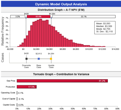
Image from the 4-D Resources article

“In the simple example (to the right), the financial model was more real-world through using input variables and correlation assumptions that reflect historical and projected reality rather than single data estimates that tend towards the most expected value.”
“Additionally, the output data provide greater insight into the variability of outcomes than the static model Downside, Base and Upside cases’ single data estimates did.”
The tornado diagram, shown below the histogram, essentially is another representation of the spider diagram information. ie.e which factors have the biggest impact.
“The dynamic data also facilitated the real option value of the asset in a manner a static model cannot. And the model took less time to build, with less internal relationships to create to make the output trustworthy, given input variables and correlation were set using the @RISK software options. This dynamic modeling approach can be used for all types of financial models.”
To read the full article, follow this link.

Conclusion

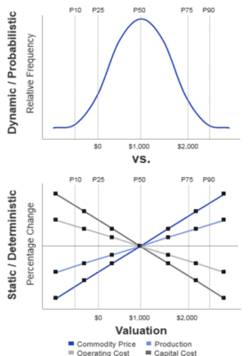
image from 4-D Resources article

Improvements are needed in the way risks are evaluated and explained to mining stakeholders. Improvements are required given increasing complexity in the risks impacting on decision making.
The probabilistic risk evaluation approach described above isn’t new and isn’t that complicated. In fact, it can be very intuitive when undertaken properly.
Probabilistic risk analysis isn’t something that should only be done within the inner sanctums of large mining companies. The approach should filter down to all mining studies and 43-101 reports.
It should ultimately become a best practice or standard part of all mining project economic analyses. The more often the approach is applied, the sooner people will become familiar (and comfortable) with it.
Mining projects can be risky, as demonstrated by the numerous ventures that have derailed. Yet recognition of this risk never seems to be brought to light beforehand.
Essentially all mining projects look the same to outsiders from a risk perspective, when in reality they are not. The mining industry should try to get better in explaining this.
Management understandably have a difficult task in making go/no-go decisions. Financial institutions have similar dilemmas when deciding on whether or not to finance a project.   You can read that blog post at this link “Flawed Mining Projects – No Such Thing as Perfection
UPDATE:  For those interesting in this subject, there is a follow up article by the same author published in January 2022 titled “Using Dynamic Financial Modeling to Enhance Insights from Financial Reports!“.
Note: You can sign up for the KJK mailing list to get notified when new blogs are posted. Follow me on Twitter at @KJKLtd for updates.
Share

Pit Optimization – More Than Just a “NPV vs RF” Graph

In this blog I wish to discuss some personal approaches used for interpreting pit optimization data. I’m not going to detail the basics of pit optimization, assuming the reader is already familiar with it .
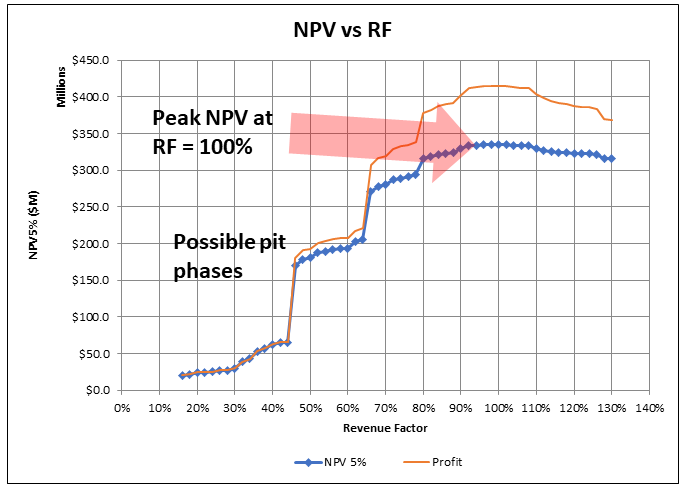
Often in 43-101 technical reports, when it comes to pit optimization, one is presented with the basic “NPV vs Revenue Factor (RF)” curve.  That’s it.
Revenue Factor represents the percent of the base case metal price(s) used to optimize for the pit. For example, if the base case gold price is $1600/oz (100% RF), then the 80% RF is $1280/oz.
The pit shell used for pit design is often selected based on the NPV vs RF curve, with a brief explanation of why the specific shell was selected. Typically it’s the 100% RF shell or something near the top of the NPV curve.
However the pit optimization algorithm generates more data than just shown in the NPV graph.  An example of that data is shown in the table below. For each Revenue Factor increment, the data for ore and waste tonnes is typically provided, along with strip ratio, NPV, Profit, Mining cost, Processing, and Total Cost at a minimum.
Luckily it is quick and easy to examine more of the data than just the NPV curve.

In many 43-101 reports, limited optimization analysis is presented.  Perhaps the engineers did drill down deeper into the data and only included the NPV graph in the report for simplicity purposes. I have sometimes done this to avoid creating five pages of text on pit optimization alone, which few may have interest in. However, in due diligence data rooms I have also seen many optimization summary files with very limited interpretation of the optimization data.
Pit optimization is a approximation process, as I outlined in a prior post titled “Pit Optimization–How I View It”. It is just a guide for pit design. One must not view it as a final and definitive answer to what is the best pit over the life of mine since optimization looks far into the future based on current information, .
The pit optimization analysis does yield a fair bit of information about the ore body configuration, the vertical grade distribution, and addresses how all of that impacts on the pit size. Therefore I normally examine a few other plots that help shed light on the economics of the orebody. Each orebody is different and can behave differently in optimization. While pit averages are useful, it is crucial to examine the incremental economic impacts between the Revenue Factor shells.

What Else Can We Look At?

The following charts illustrate the types of information that can be examined with the optimization data. Some of these relate to ore and waste tonnage. Some relate to mining costs. Incremental strip ratios, especially in high grade deposits, can be such that open pit mining costs (per tonne of ore) approach or exceed the costs of underground mining. Other charts relate to incremental NPV or Profit per tonne per Revenue Factor.  (Apologies if the chart layout below appears odd…responsive web pages can behave oddly on different devices).

Conclusion

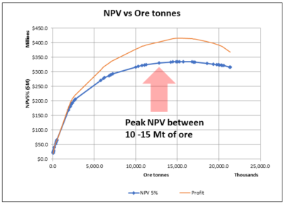
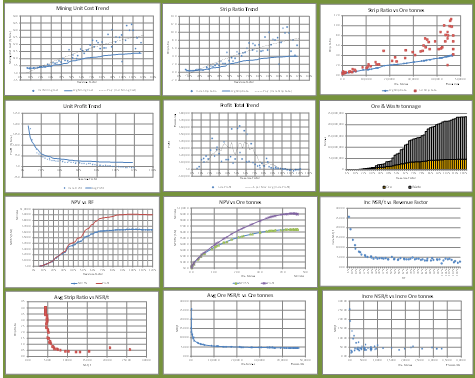
It’s always a good idea to drill down deeper into the optimization output data, even if you don’t intend to present that analysis in a final report. It will help develop an understanding of the nature of the orebody.
It shows how changes in certain parameters can impact on a pit size and whether those impacts are significant or insignificant. It shows if economics are becoming very marginal at depth. You have the data, so use it.
This discussion presents my views about optimization and what things I tend to look at.   I’m always learning so feel free to share ways that you use your optimization analysis to help in your pit design decision making process.
As referred to earlier, there is a lot of uncertainty in the input parameters used in open pit optimization.  These might include costs, recoveries, slope angles and other factors.  If you would like to read more, the link to that post is here.  “Pit Optimization–How I View It”.
Note: You can sign up for the KJK mailing list to get notified when new blogs are posted. Follow me on Twitter at @KJKLtd for updates.
Share

Are Engineers Too Pessimistic

Geological colleagues have often joked that engineers are a pessimistic lot; they are never technically satisfied. The engineers will fire back that geologists are an overly optimistic lot; every speck of mineralization makes them ecstatic. Together they make a great team since each cancels the other out.
In my opinion engineers are often pessimistic. This is mainly because they have been trained to be that way. Throughout my own engineering career I have been called upon many times to focus on the downsides, i.e. what can happen that we don’t want to happen.

It starts early and continues on

This pessimism training started early in my career while working as a geotechnical engineer. Geotechnical engineers were always looking at failure modes and the potential causes of failure when assessing factors of safety.
Slope failure could be due to the water table, excess pore pressures, seismic or blast vibrations, liquefaction, unknown weak layers, overly steepen slopes, or operating error. As part of our job we had to come up with our list of negatives and consider them all. The more pessimistic view you had, the better job you did.
This training continued through the other stages of a career. The focus on negatives continues in mine planning and costing.
For example, there are 8,760 hours in a year, but how many productive hours will each piece of equipment provide? There will delays due to weather conditions, planned maintenance, unplanned breakdowns, inter-equipment delays, operator efficiency, and other unforeseen events. The more pessimistic a view of equipment productivity, the larger the required fleet. Geotechnical engineers would call this the factor of safety.
In the more recent past, I have been involved in numerous due diligences. Some of these were done for major mining companies looking at acquisitions. Others were on behalf of JV partners, project financiers, and juniors looking at acquisitions.
When undertaking a due diligence, particularly for a major company or financier, we are not hired to tell them how great the project is. We are hired to look for fatal flaws, identify poorly based design assumptions or errors and omissions in the technical work. We are mainly looking for negatives or red flags.
Often we get asked to participate in a Risk Analysis or SWOT analysis (Strengths-Weaknesses-Opportunities-Threats) where we are tasked with identifying strengths and weaknesses in a project.
Typically at the end of these SWOT exercises, one will see many pages of project risks with few pages of opportunities.
The opportunities will usually consist of the following cliches (feel free to use them in your own risk session); metal prices may be higher than predicted; operating costs will be lower than estimated; dilution will be better than estimated; and grind size optimization will improve process recoveries.
The project’s risk list will be long and have a broad range. The longer the list of risks, the smarter the review team appears to be.

Investing isn’t easy

After decades of the training described above, it becomes a challenge for me to invest in junior miners. My skewed view of projects carries over into my investing approach, whereby I tend to see the negatives in a project fairly quickly. These may consist of overly optimistic design assumptions or key technical aspects not understood in sufficient depth.
Most 43-101 technical reports provide a lot of technical detail; however some of them will still leave me wanting more. Most times some red flags will appear when first reviewing these reports. Some of the red flags may be relatively inconsequential or can be mitigated. However the fact that they exist can create concern. I don’t know if management knows they exists or knows how they can mitigate them.
It has been my experience that digging in a data room or speaking with the engineering consultants can reveal issues not identifiable in a 43-101 report. Possibly some of these issues were mentioned or glossed over in the report, but you won’t understand the full extent of the issues until digging deeper.
43-101 reports generally tell you what was done, but not why it was done. The fact I cannot dig into the data room or speak with the technical experts is what has me on the fence. What facts might I be missing?
Statistics show that few deposits or advanced projects become real mines. However every advanced study will say that this will be an operating mine. Many projects have positive feasibility studies but these studies are still sitting on the shelf. Is the project owner a tough bargainer or do potential acquirers / financiers see something from their due diligence review that we are not aware of?   You don’t get to see these third party reviews unless you have access to the data room.
My hesitance in investing in some companies unfortunately can be penalizing. I may end up sitting on the sidelines while watching the rising stock price. Junior mining investors tend to be a positive bunch, when combined with good promotion can result in investors piling into a stock.
Possibly I would benefit by putting my negatives aside and instead ask whether anyone else sees these negatives. If they don’t, then it might be worth taking a chance, albeit making sure to bail out at the right time.
Often newsletter writers will recommend that you “Do your own due diligence”. Undertaking a deep dive in a company takes time. In addition I’m not sure one can even do a proper due diligence without accessing a data room or the consulting team. In my opinion speaking with the engineering consultants that did the study is the best way to figure things out. That’s one reason why “hostile” due diligences can be difficult, while “friendly” DD’s allow access to a lot more information.

Conclusion

Sometimes studies that I have been involved with have undergone third party due diligence. Most times one can predict ahead of time which issues will be raised in the review. One knows how their engineers are going to think and what they are going to highlight as concerns.
Most times the issue is something we couldn’t fully address given the level of study. We might have been forced to make best guess assumptions to move forward. The review engineers will have their opinions about what assumptions they would have used. Typically the common comment is that our assumption is too optimistic and their assumption would have been more conservative or realistic (in their view).
Ultimately if the roles were reversed and I were reviewing the project I may have had the same comments. After all, the third party reviewers aren’t being hired to say everything is perfect with a project.
The odd time one hears that our assumption was too pessimistic. You usually hear this comment when the reviewing consultant wants to do the next study for the client. They would be a much more optimistic and accommodating team.
To close off this rambling blog, the next time you feel that your engineers are too negative just remember that they are trained to be that way.  If you want more positivity, hang out with a geologist (or hire a new grad).


Note: You can sign up for the KJK mailing list to get notified when new blogs are posted. Follow me on Twitter at @KJKLtd for updates and insights.
Share

Pre-Concentration – Maybe Good, Maybe Not

A while back I wrote a blog titled “Pre-Concentration – Savior or Not?”. That blog was touting the benefits of pre-concentration. More recently I attended a webinar where the presenter stated that the economics of pre-concentration may not necessarily be as good as we think they are.
My first thought was “this is blasphemy”. However upon further reflection I wondered if it’s true. To answer that question, I modified one of my old cashflow models from a Zn, Pb project using pre-concentration. I adjusted the model to enable running a trade-off, with and without pre-con by varying cost and recovery parameters.

Main input parameters

The trade-off model and some of the parameters are shown in the graphic below. The numbers used in the example are illustrative only, since I am mainly interested in seeing what factors have the greatest influence on the outcome.

The term “mass pull” is used to define the quantity of material that the pre-con plant pulls and sends to the grinding circuit. Unfortunately some metal may be lost with the pre-con rejects.  The main benefit of a pre-con plant is to allow the use of a smaller grinding/flotation circuit by scalping away waste. This will lower the grinding circuit capital cost, albeit slightly increase its unit operating cost.
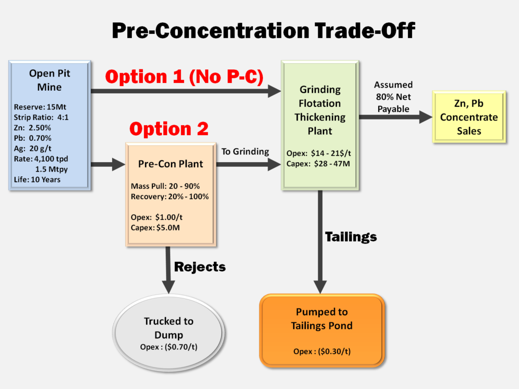
Concentrate handling systems may not differ much between model options since roughly the same amount of final concentrate is (hopefully) generated.
Another one of the cost differences is tailings handling. The pre-con rejects likely must be trucked to a final disposal location while flotation tails can be pumped.  I assumed a low pumping cost, i.e to a nearby pit.
The pre-con plant doesn’t eliminate a tailings pond, but may make it smaller based on the mass pull factor. The most efficient pre-concentration plant from a tailings handling perspective is shown on the right.

The outcome

The findings of the trade-off surprised me a little bit.  There is an obvious link between pre-con mass pull and overall metal recovery. A high mass pull will increase metal recovery but also results in more tonnage sent to grinding. At some point a high mass pull will cause one to ask what’s the point of pre-con if you are still sending a high percentage of material to the grinding circuit.
The table below presents the NPV for different mass pull and recovery combinations. The column on the far right represents the NPV for the base case without any pre-con plant. The lower left corner of the table shows the recovery and mass pull combinations where the NPV exceeds the base case. The upper right are the combinations with a reduction in NPV value.
The width of this range surprised me showing that the value generated by pre-con isn’t automatic.  The NPV table shown is unique to the input assumptions I used and will be different for every project.

The economic analysis of pre-concentration does not include the possible benefits related to reduced water and energy consumption. These may be important factors for social license and permitting purposes, even if unsupported by the economics.  Here’s an article from ThermoFisher on this “How Bulk Ore Sorting Can Reduce Water and Energy Consumption in Mining Operations“.

Conclusion

The objective of this analysis isn’t to demonstrate the NPV of pre-concentration. The objective is to show that pre-concentration might or might not make sense depending on a project’s unique parameters. The following are some suggestions:
1. Every project should at least take a cursory look at pre-concentration to see if it is viable. This should be done on all projects, even if it’s only a cursory mineralogical assessment level.
2. Make certain to verify that all ore types in the deposit are amenable to the same pre-concentration circuit. This means one needs to have a good understanding of the ore types that will be encountered.
3. Anytime one is doing a study using pre-concentration, one should also examine the economics without it. This helps to understand the  economic drivers and the risks. You can then decide whether it is worth adding another operating circuit in the process flowsheet that has its own cost and performance risk. The more processing components added to a flow sheet, the more overall plant availability may be effected.
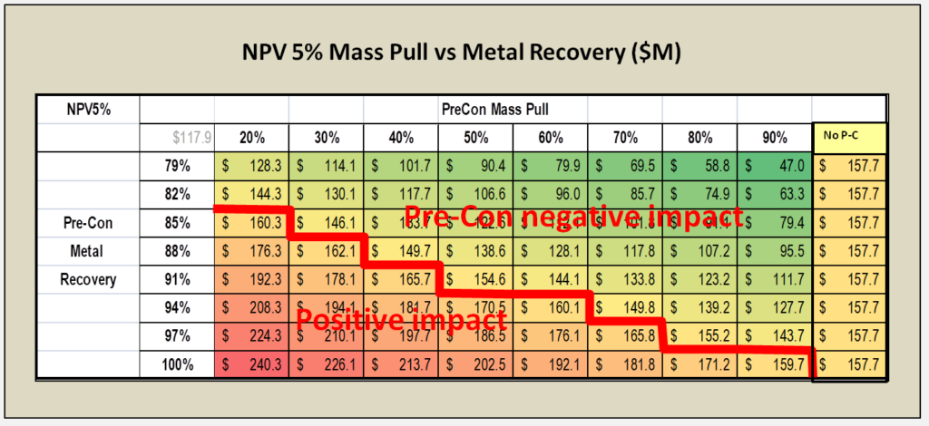
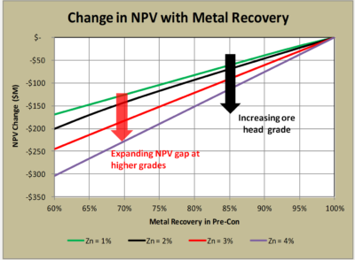
4. The head grade of the deposit also determines how economically risky pre-concentration might be. In higher grade ore bodies, the negative impact of any metal loss in pre-concentration may be offset by accepting higher cost for grinding (see chart on the right).
5. In my opinion, the best time to decide on pre-con would be at the PEA stage. Although the amount of testing data available may be limited, it may be sufficient to assess whether pre-con warrants further study.
6. Don’t fall in love with or over promote pre-concentration until you have run the economics. It can make it harder to retract the concept if the economics aren’t there.


Note: You can sign up for the KJK mailing list to get notified when new blogs are posted.
Follow us on Twitter at @KJKLtd for updates and insights.
Share

Climbing the Hill of Value With 1D Modelling

Recently I read some articles about the Hill of Value.  I’m not going into detail about it but the Hill of Value is a mine optimization approach that’s been around for a while.  Here is a link to an AusIMM article that describes it “The role of mine planning in high performance”.  For those interested, here is a another post about this subject “About the Hill of Value. Learning from Mistakes (II)“.
hill of value

(From AusIMM)

The basic premise is that an optimal mining project is based on a relationship between cut-off grade and production rate.  The standard breakeven or incremental cutoff grade we normally use may not be optimal for a project.
The image to the right (from the aforementioned AusIMM article) illustrates the peak in the NPV (i.e. the hill of value) on a vertical axis.
A project requires a considerable technical effort to properly evaluate the hill of value. Each iteration of a cutoff grade results in a new mine plan, new production schedule, and a new mining capex and opex estimate.
Each iteration of the plant throughput requires a different mine plan and plant size and the associated project capex and opex.   All of these iterations will generate a new cashflow model.
The effort to do that level of study thoroughly is quite significant.  Perhaps one day artificial intelligence will be able to generate these iterations quickly, but we are not at that stage yet.

Can we simplify it?

In previous blogs (here and here) I described a 1D cashflow model that I use to quickly evaluate projects.  The 1D approach does not rely on a production schedule, instead uses life-of-mine quantities and costs.  Given its simplicity, I was curious if the 1D model could be used to evaluate the hill of value.
I compiled some data to run several iterations for a hypothetical project, loosely based on a mining study I had on hand.  The critical inputs for such an analysis are the operating and capital cost ranges for different plant throughputs.
hill of value
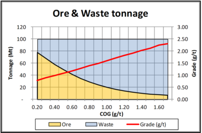
I had a grade tonnage curve, including the tonnes of ore and waste, for a designed pit.  This data is shown graphically on the right.   Essentially the mineable reserve is 62 Mt @ 0.94 g/t Pd with a strip ratio of 0.6 at a breakeven cutoff grade of 0.35 g/t.   It’s a large tonnage, low strip ratio, and low grade deposit.  The total pit tonnage is 100 Mt of combined ore and waste.
I estimated capital costs and operating costs for different production rates using escalation factors such as the rule of 0.6 and the 20% fixed – 80% variable basis.   It would be best to complete proper cost estimations but that is beyond the scope of this analysis. Factoring is the main option when there are no other options.
The charts below show the cost inputs used in the model.   Obviously each project would have its own set of unique cost curves.
The 1D cashflow model was used to evaluate economics for a range of cutoff grades (from 0.20 g/t to 1.70 g/t) and production rates (12,000 tpd to 19,000 tpd).  The NPV sensitivity analysis was done using the Excel data table function.  This is one of my favorite and most useful Excel features.
A total of 225 cases were run (15 COG versus x 15 throughputs) for this example.

What are the results?

The results are shown below.  Interestingly the optimal plant size and cutoff grade varies depending on the economic objective selected.
The discounted NPV 5% analysis indicates an optimal plant with a high throughput (19,000 tpd ) using a low cutoff grade (0.40 g/t).  This would be expected due to the low grade nature of the orebody.  Economies of scale, low operating costs, high revenues, are desired.   Discounted models like revenue as quickly as possible; hence the high throughput rate.
The undiscounted NPV 0% analysis gave a different result.  Since the timing of revenue is less important, a smaller plant was optimal (12,000 tpd) albeit using a similar low cutoff grade near the breakeven cutoff.
If one targets a low cash cost as an economic objective, one gets a different optimal project.  This time a large plant with an elevated cutoff of 0.80 g/t was deemed optimal.
The Excel data table matrices for the three economic objectives are shown below.  The “hot spots” in each case are evident.

hill of value

hill of value

Conclusion

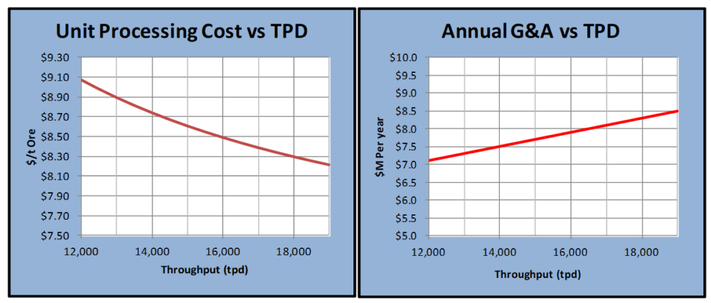
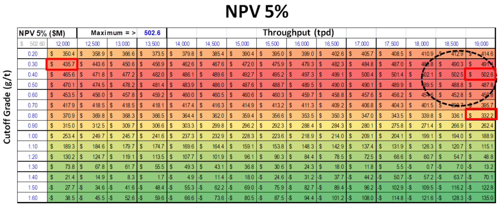
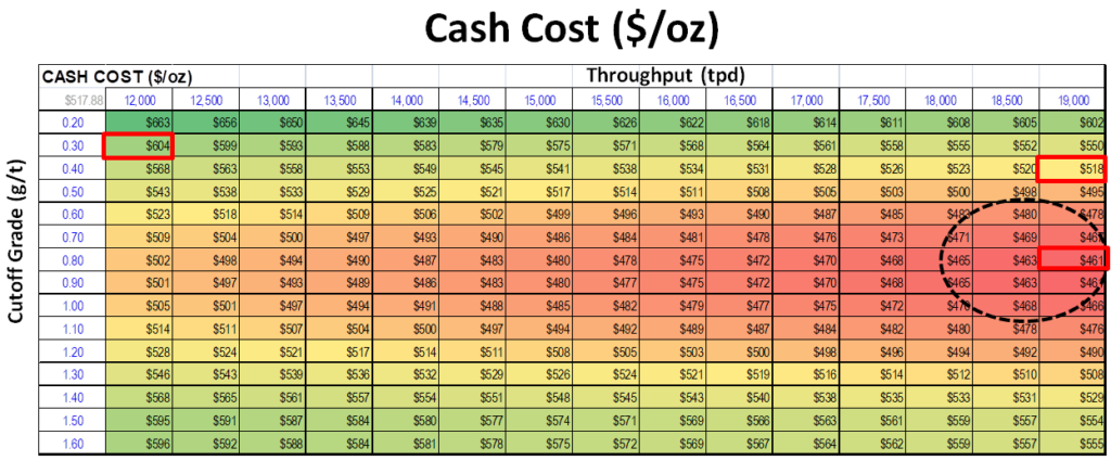
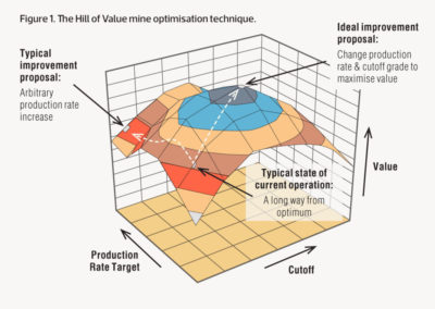
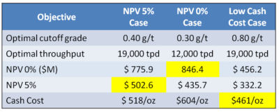
The Hill of Value is an interesting optimization concept to apply to a project.  In the example I have provided, the optimal project varies depending on what the financial objective is.  I don’t know if this would be the case with all projects, however I suspect so.
In this example, if one wants to be a low cash cost producer, one may have to sacrifice some NPV to do this.
If one wants to maximize discounted NPV, then a large plant with low opex would be the best alternative.
If one prefers a long mine life, say to take advantage of forecasted upticks in metal prices, then an undiscounted scenario might win out.
I would recommend that every project undergoes some sort of hill of value test, preferably with more engineering rigor. It helps you to  understand a projects strengths and weaknesses.  The simple 1D analysis can be used as a guide to help select what cases to look at more closely. Nobody wants to assess 225 alternatives in engineering detail.
In reality I don’t ever recall seeing a 43-101 report describing a project with the hill of value test. Let me know if you are aware of any, I’d be interested in sharing them.  Alternatively, if you have a project and would like me to test it on my simple hill of value let me know.
Note: You can sign up for the KJK mailing list to get notified when new blogs are posted.
Share

Benchmarking – Let’s See More Of It

Benchmarking is the process of measuring performance of a company’s attributes against those of another. Ideally the benchmarking comparison is made against what are considered to be the best in the industry.  Sometimes however the comparison is simply made between industry peers.
We often see junior mining companies benchmarking themselves against others. Sometimes corporate presentations provide graphs of enterprise value per gold ounce to demonstrate that a company might be undervalued.
We also see cash cost charts (an example to the right) benchmarking where a company’s production cost will rank among its competitors.
I view benchmarking as a great thing. The information can be very insightful, but with the caveat that it takes effort to ensure the comparative data is accurate.

Can we see more benchmarking?

Given the benefits of benchmarking, another area that might warrant such effort is related to capital cost estimates.
When a project moves into the development stage, the first two observable metrics are the construction progress and the capital cost expenditures. The capital cost trend is generally given very close scrutiny since it is a key indicator describing where a project is heading.
Lenders may have observers at site monitoring both construction progress and cash expenditures. Shareholders and analysts are watching for news releases that update the capital spending. Their concern is well founded due to several significant cost over-run instances.
Some of these over-runs have been fatal whereby the company has been unable to secure additional financing for the extra costs. There are others instances where a financing white knight has come in and essentially wrestled company ownership away from current shareholders.
Some industry people also feel that capital cost performance can foreshadow a project’s performance once it goes into commercial production.
Capital cost over-runs may be caused by poor execution and/or unforeseen events, or due to inaccurate cost estimation to begin with.  Many investors still have apprehension with capital cost estimates from advanced studies. This is where benchmarking may play a role. Mining company shareholders may want to see a comparison of their project capital cost with other similar projects.

Project databases

It would be a good thing if the mining industry (or other concerned parties) work together to create open source project databases. These would incorporate summary information and cost information for global mining projects.  The information is already out there, it just needs to be compiled.
One nice thing is that younger workers coming into the mining industry exhibit an interest in collaboration and information sharing. Hence maintaining the databases could be done by interested parties, industry experts, and/or crowd sourcing.
The databases would be public domain accessible to everyone and  could be used to benchmark a project against other similar projects.  The Global Tailings Portal (tailing.grida.no/about) is working to build a freely accessible database for the thousands of tailings dam globally. Its the same idea.
I realize that many mining projects are unique with site specific features and conditions. However many projects are also very similar to one another. For example West African gold projects in many cases can be replicates of one another with similar capital costs.
Published technical reports could include a chapter on benchmarking, whereby a project is compared with other similar projects. A company could provide rationale why their project will be costlier (or less expensive) than the others.

Conclusion

Benchmarking can be a great tool when done correctly. Benchmarking  capital costs might bring more transparency to the project development process. It may help convince nervous investors that the proposed costs are reasonable.
We already see corporate presentations using benchmarking, so why stop at production costs and share price valuation.
One could expand the reach to include operating costs but internal confidentiality may be an issue.  Furthermore operating costs are longer in duration and subject to change with global influences.
Capital cost accuracy is one of the primary concerns in the development of new projects. Possibly more benchmarking is part of the solution.


Note: You can sign up for the KJK mailing list to get notified when new blogs are posted.
Share

Do Any Junior Producers Model a Gold ETF?

junior mining company
I have often wondered if any of the smaller gold producers have ever considered modelling their business plan similar to a gold Exchange Traded Fund (“ETF”).
This hybrid business model may be a way for companies to provide shareholders a way to leverage themselves to physical gold rather than leveraging to the performance of a mine.

Let me explain further

Consider two identical small mining companies each starting up a new mine. Their projects are identical; 2 million gold ounces in reserves with annual production rate of 200,000 ounces with a 10 year mine life. On an annual basis, let’s assume their annual operating costs and debt repayments could be paid by the revenue from selling 180,000 ounces of gold. This would leave 20,000 gold ounces as “profit”. The question is what to do with those 20,000 ounces?

Gold Dore

Company A

Company A sells their entire gold production each year. At $1200/oz, the 20,000 oz gold “profit” would yield $24 million. Income taxes would be paid on this and the remaining cash can be spent or saved.
Company A may decide to spend more on head offices costs by adding more people, or they may spend money on exploration, or they could look at an acquisition to grow the company. There are plenty of ways to use this extra money, but returning it to shareholders as a dividend isn’t typically one of them.
Now let’s jump forward several years; 8 years for example. Company A may have been successful on grassroots exploration and added new reserves but historically exploration odds are working against them. If they actually saved a portion of the annual profit, say $10M of the $24M, after 8 years they may have $80M in cash reserves.

Company B

Company B only sells 180,000 ounces of gold each year to cover costs.  It puts the remaining 20,000 ounces into inventory. Their annual profit-loss statement shows breakeven status since their gold sales only cover their financial commitments. In this scenario, after 8 years Company B would have 160,000 gold ounces in inventory, valued at $192 million at a $1200 gold price.
If you’re an investor looking at both these companies in the latter stages of their mine life, which one would you rather invest in?
Company A has 400,000 ounces (2 years) remaining in mineral reserves and $80M cash in the bank. Company B also has 400,000 ounces of mineral reserves and $192 million worth of gold in the vault. If I’m a bullish gold investor and foresee a $1600/oz gold price, then to me Company B might theoretically have $256M in the vault (160k oz x $1600). If I’m a super bullish, their gold inventory could be worth a lot more..theoretically.

Which company is worth more?

I assume that the enterprise value (and stock price) of Company A would be based on its remaining reserves at some $/oz factor plus its cash in the bank. Company B could be valued the same way plus its gold inventory. So for me Company B may be a much better investment than Company A in the latter stages of its mine life. In fact Company B could still persist as an entity after the mine has shutdown simply as a “fund” that holds physical gold. If I am a gold investor, then Company B as an investment asset might be of more interest to me.
If Company A had good exploration results and spend money wisely, then it may have more value but not all companies are successful down this path.

Conclusion

It appears that most of the time companies sell their entire annual gold production to try to show profit on the annual income statement. This puts cash in the bank and shows “earning per share”.
My question is why not stockpile the extra gold and wait for gold prices to rise?  This might be an option if the company doesn’t really need the money now or doesn’t plan to gamble on exploration or acquisitions.
This concept wouldn’t be a model for all small miners but might be suitable for a select few companies to target certain types of gold investors.
They could provide an alternative mining investment that might be especially interesting in the last years of a mine life. Who really wants to buy shares in a company who’s mine is nearly depleted?  I might buy shares, if they still hold a lot of gold.
Note: You can sign up for the KJK mailing list to get notified when new blogs are posted.
Share

Higher Metal Prices – Should Miners Lower the Cut-Off Grade?

When metals prices are high, we are generally told that we should lower the cutoff grade. Our cutoff grade versus metal price formula tells us this is the correct thing do. Our grade-tonnage curve reaffirms this since we will now have more metal in the mineral reserve.

But is lowering the cutoff grade the right thing?

Books have been written on the subject of cutoff grades where readers can get all kinds of detailed logic and calculations using Greek symbols (F = δV* − dV*/dT). Here is one well known book by Ken Lane, available on Amazon HERE.
Recently we have seen a trend of higher cash costs at operating mines when commodity prices are high. Why is this?
It may be due to higher cost operating inputs due to increasing labour rates or supplies. It may also be partly due to the lowering of cutoff grades.  This lowers the head grade, which then requires more tonnes to be milled to produce the same quantity of metal.
A mining construction manager once said to me that he never understood us mining guys who lower the cutoff grade when gold prices increase. His concern was that since the plant throughput rate is fixed, when gold prices are high we suddenly decide to lower the head grade and produce fewer and higher cost ounces of gold.

Do the opposite

His point was that we should do the opposite.  When prices are high, we should produce more ounces of gold, not fewer. In essence, periods when supply is low (or demand is high) may not be the right time to further cut  supply by lowering head grades.
Now this is the point where the grade-tonnage curve comes into play.
Certainly one can lower the cutoff grade, lower the head grade and produce fewer ounces of gold.  The upside being an extension in the mine life.  A company can report more ounces in reserves and perhaps the overall image of the company looks better (if it is being valued on reserves).   To read more about the value of grade-tonnage curves, you check out this blog post “Grade-Tonnage Curves – Worthy of a Good Look.

What if metal prices drop back?

The problem is that there is no guarantee that metal prices will remain where they are and the new lower cutoff grade will remain where it is. If the metal prices drop back down, the cutoff grade will be increased and the mineral reserve will revert back to where it was. All that was really done was accept a year of lower metal production for no real long term benefit.
This trade-off  contrasts a short term vision (i.e. maximizing annual production) against a long term vision (i.e. extending mineral reserves).

Conclusion

The bottom line is that there is no simple answer on what to do with the cutoff grades.  Hence there is a need to write books about it.
Different companies have different corporate objectives and each mining project will be unique with regards to the impacts of cutoff grade changes on the orebody.
I would like to caution that one should be mindful when plugging in new metal prices, and then running off to the mine operations department with the new cutoff grade. One should fully understand both the long term and short term impacts of that decision.
In another blog post on the cutoff grade issue, I discuss whether in poly-metallic deposits the cutoff should be based on metal equivalent or block NSR value.  Neither approach is perfect, but I prefer the NSR option.  You can read that post at “Metal Equivalent Grade versus NSR for Poly-Metallics“.


Note: If you would like to get notified when new blogs are posted, then sign up on the KJK mailing list on the website.  Otherwise I post notices on LinkedIn, so follow me at: https://www.linkedin.com/in/kenkuchling/.
Share