


Rarely do you see both the table and curve in the report, although ideally one would want to see both. Given the option, I would prefer to see the graph more than the table of numbers. The trend of the grade-tonnage information is just as important as the values, maybe even a bit more important. Unfortunately, a data table by itself doesn’t illustrate trends very well.
Useful Grade-Tonnage Curve Information
 When I am undertaking a due diligence review or working on a study, very early on I like to have a look at the grade-tonnage information. This could be for the entire deposit resource, within a resource constraining shell, or in the pit design.
The grade-tonnage information gives an understanding of how future economics or technical issues may impact on the mineable tonnage.
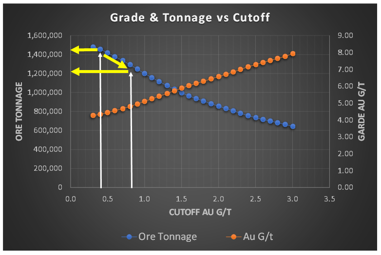
An example of a typical grade-tonnage curve is shown here.
The cutoff grade along the x-axis will be impacted by changes in metal price or operating cost. The cutoff grade will increase if metal prices decrease or if operating costs increase.
The question is how sensitive is the mineable tonnage to these economic factors. The slope of the tonnage and grade curves will help answer this question.
In the example shown, the tonnage curve (blue dots) is fairly linear, meaning the ore tonnage steadily decreases with increasing cut-off grade. That is expected and is reasonable.
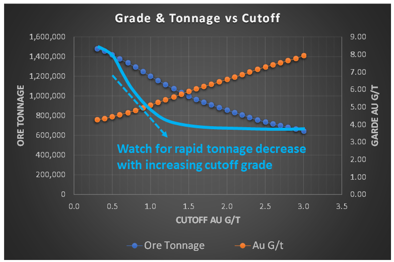 However, if the tonnage curve profile resembled the light blue line in this image, with a concave shape, the ore tonnage is decreasing rapidly with increasing cutoff grade. This is generally not a favorable situation.
It indicates that a significant portion of the tonnage has a grade close to the cutoff grade. If that’s the situation, the calculation of the cutoff and the inputs used to generate it are important and worthy of scrutiny. Are they reasonable? Over the long term, is the cutoff grade more likely to increase or decrease?
The same logic can be used with the ore grade curve in the graph. As shown in this example, the ore grade increases steadily as the cutoff is raised. This is because lower grade ore is being shifted from ore to waste, and hence the remaining ore has better quality. If the cutoff is raised from 0.4 g/t to 0.5 g/t, then some material with a grade of about 0.45 g/t is moved from ore to waste.
I also like to compare the ratio of the average grade to the cutoff grade. Its nice to see a ratio of 4:1 to 5:1 to ensure the overall average grade isn’t close to the cutoff. In this example, the cutoff grade is 0.5 g/t and the average grade is 4.5 g/t, a ratio of 9:1.
The tonnage curve and grade curve provide information on the nature of the mineral resource. Study them both.
Reporting Waste Within a Shell
 One complaint I have about reporting mineral resources inside a resource constraining shell is the lack of strip ratio information. This applies whether disclosing a single mineral resource estimate or variable grade-tonnage data.
In my view, the strip ratio is even more important to be aware of when looking at grade tonnage data.
The strip ratio within a shell will climb as an increasing cutoff grade results in a decreasing ore tonnage. Sometimes the strip ratio will increase exponentially. The corresponding amount of waste remaining in that pit shell increases, hence the ratio of the two (i.e. strip ratio) can escalate rapidly.
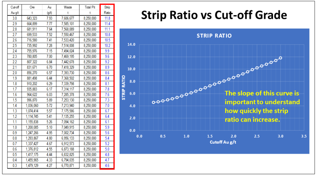 Regarding mineral resources, one should be required to disclose the waste tonnage and strip ratio when reporting resources inside a constraining shell. The constraining shell and cutoff grade are both based on defined economic factors such as unit mining costs, processing cost, process recoveries, and metal prices. With respect to the mining cost component, the strip ratio is a key aspect of the total mining cost, yet it normally isn’t disclosed.
Its common to see mention that the mining cost is (say) $2.50/t, but if the strip ratio is 10:1, that equates to an effective mining cost of $27.50 per tonne of ore. That’s an important cost to know, especially if one is pushing a pit shell deep to maximum the mineral resource tonnage.
Each mineral deposit resource model can behave differently. Hence, in my view, the waste tonnage should be included when reporting mineral resource tonnages (or presenting grade-tonnage data) within a constraining shell. This waste tonnage or strip ratio can be in the footnotes to the mineral resource summary table.
Spider Diagram Downsides
 In 43-101 technical reports, the financial Chapter 22 normally presents the project sensitivities expressed in a spider diagram or a table format.
In a previous blog post I had discussed the flaws in the spider diagram approach. That article link is at “Cashflow Sensitivity Analyses – Be Careful”. The grade-tonnage curve helps explain why that is.
In the spider diagrams, we typically see sensitivities related to +/- 20% on metal prices and operating costs. If either of these factors change, then in reality the cutoff grade would change.
If the metal price decreases by -20%, or the operating cost climbs by +20%, the cutoff grade must increase. This adjustment is normally not made in the sensitivity analysis because it requires a lot of re-work.
Elevating the cutoff grade would shift the pit ore tonnage towards the right on the grade-tonnage curve, showing a decrease in mineable tonnes. However, in the spider diagram logic, the assumption is that production schedule in the cashflow model is unchanged and simply the metal prices or operating costs are adjusted. Therefore, the spider diagram can be a misleading representation of the downside risk, showing a more positive situation than in reality.
Conclusion
