Articles tagged with: PEA

The Double Life of Inferred Resources: Now You See It – Now You Don’t

Date: April 18, 2026 Author: Ken Kuchling Comments: Leave a reply

There is a unique paradox sitting at the heart of how the mining industry evaluates its projects. It’s called the Inferred Resource—now you see it, now you don’t.

A company can publish a Preliminary Economic Assessment (PEA) showing a mine life, a robust internal rate of return, and a strong net present value. That study can be based on mineral resources that regulators consider too geologically uncertain to support a production decision. These are the infamous Inferred resources: tonnes, grades, and dollars in the economic model, yet with a classification that effectively flags them as educated guesses. The PEA rules permit their inclusion because early-stage projects need a way to test whether chasing more resource certainty is worth the additional cost.

The paradox occurs when that same project advances to the pre-feasibility (PFS) or feasibility (FS) stage. Suddenly the Inferred ore tonnes are gone; they are now waste rock. The mine plan must be based on more certain Measured and Indicated resources. Theoretically, the life-of-mine production profile that looked compelling in the PEA may now shrink—so the NPV and IRR might shrink too. Nothing has gone wrong in any technical sense. The project simply requires a higher standard of certainty now.

Potentially, some investors who focused on the PEA economics may feel the subsequent feasibility study is a disappointment (especially if costs have also escalated). They’ll say the PEA is garbage. In reality, the project has moved from an aspirational study (i.e., the PEA) toward a bank-financeable study. To compensate for the loss of Inferred material, companies will rely of step out drilling to grow the resource to maintain size.

What Are Inferred Resources?

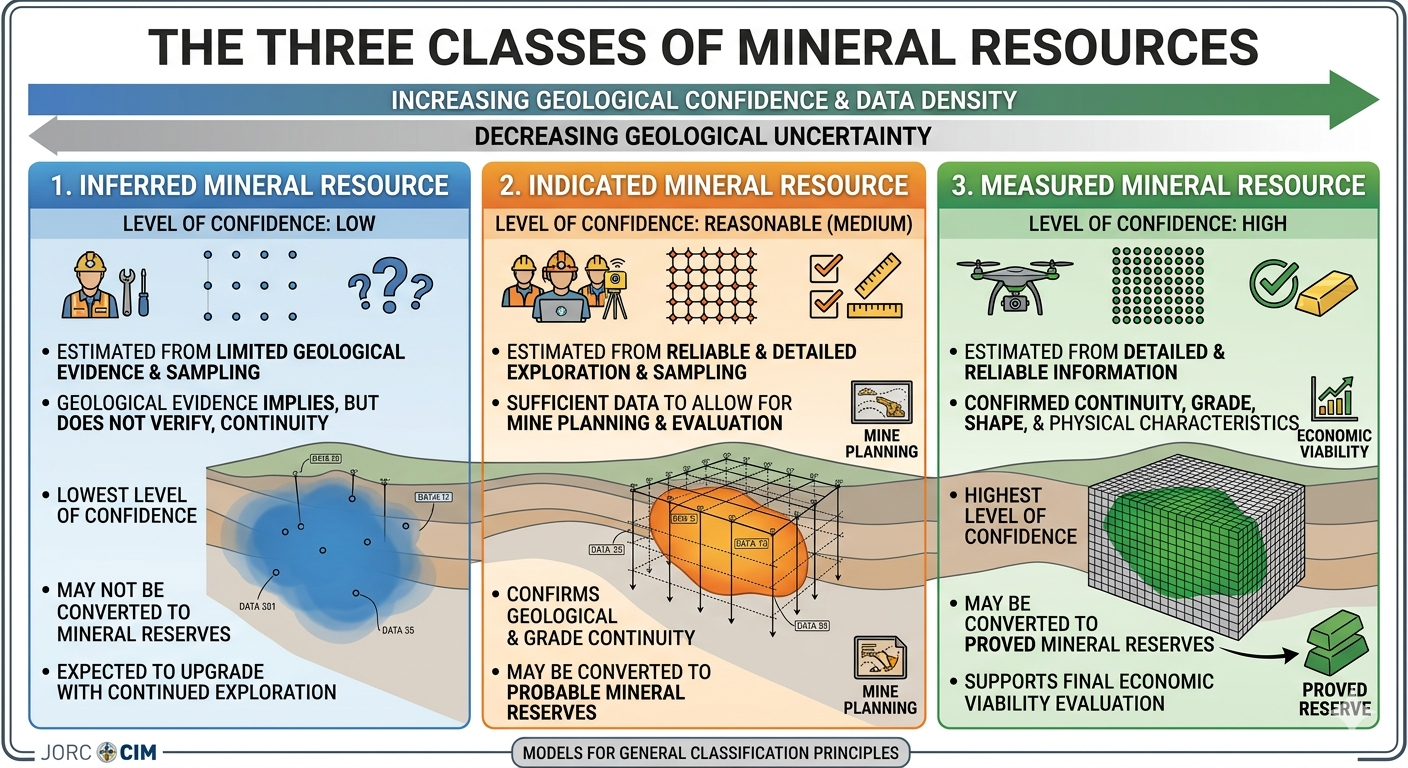Inferred resources represent the lowest confidence category of mineral resources; typically estimated in zones with limited sampling and unconfirmed geological continuity. They carry the highest geological uncertainty of the three resource categories.

In Preliminary Economic Assessments (PEAs), Inferred resources are allowed—but only under certain conditions:

They can be included in mine plans and economic models, which is the reason PEAs exist: to allow early-stage projects to test economic viability using all available resource data.
However, any PEA that includes Inferred resources cannot be used to support a production decision and must carry prominent cautionary language. Under NI 43-101, the technical report must explicitly state that the PEA is preliminary in nature, that Inferred resources are too speculative geologically to have economic considerations applied, and that there is no certainty the PEA will be realized. (It seems a PEA without Inferred resources can be used to support a production decision.)
Inferred tonnes are routinely used to extend mine life or improve project economics in PEA studies. Investors must understand this risk and should examine the proportion of mined tonnage that is classified as Inferred. This breakdown is normally presented in the Technical Report.

Conversely, in Pre-Feasibility Studies (PFS) and Feasibility Studies (FS), the rules for Inferred material are different:

Inferred resources cannot be included in mineral reserve estimates or in the economic analysis underpinning a PFS or FS. Inferred “ore” is treated as waste rock.
Only Indicated and Measured resources can be converted to Probable and Proven mineral reserves.
Including Inferred material in a PFS mine plan would typically disqualify the study from being used for project financing or a production decision.
Some companies might include Inferred material in a PFS as “upside” or as a sensitivity case, but that analysis must be clearly distinguished from the base case.

The resource upgrade requirement (from Inferred to Indicated) creates some interesting dynamics:

Companies may need additional funds to drill sufficiently to upgrade the resource before advancing to the PFS/FS stage. The cost and time for this infill drilling can be a major driver of exploration spending and can delay project timelines. Mining projects can take a long time to develop, and this is one reason why.
Companies will look at ways to compensate for the Inferred material deduction. Cutoff grade changes and step out drilling are ways to mitigate this impact.
A large Inferred resource that cannot be upgraded without great cost (due to depth, remoteness, or lack of ore-zone continuity) can permanently stall a project at the PEA stage. Hence, one may see multiple PEAs completed on the same project (i.e., the PEA loop).
In closing, the peculiarity of the Inferred resource is that it is essentially a tiered permission structure. Inferred resources are useful for early economic screening, but they must be converted to higher-confidence categories before they can support a bankable study or project debt financing.

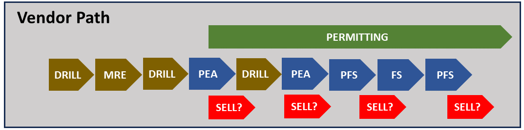
Permitting via a PEA

Companies sometimes will commence the permitting process based on their PEA study. There are some risks to doing this, and the Inferred resource creates one of these risks.

With limited capital, a junior miner may not be able to afford the $5–20 million cost of a full feasibility study before determining whether a project is even permittable. A PEA, costing a fraction of a FS, can provide enough technical substance to engage regulators and begin the environmental baseline work that must precede any formal permit application.

Baseline studies for hydrology, ecology, and air quality typically require two to three years of data collection. So starting early makes sense, even with only a PEA-level project layout in hand.

Permitting and ongoing technical study work will run in parallel on most projects. Waiting for a completed FS before starting permitting would add years to the project timeline. Companies routinely will concurrently advance environmental impact assessments, indigenous consultation, and baseline data collection with subsequent PFS and FS work.

Jurisdiction may play a role too. Some areas are more receptive to early-stage permitting engagement. Other permitting processes may be more rigorous such that operators want at least a PFS in hand before committing to a full EIA process.

Now, with respect to the Inferred resource, the risk is that a project permitted around a PEA-scale footprint may shrink in size at the feasibility stage. Some reasons for this size reduction will be discussed in a future blog post, as well as the ways companies avoid this with ever increasing ore tonnage. Project shrinkage can result in a company acquiring permits and bonding for a proposed mine plan that no longer exists.

How Can Inferred Resources Affect Permitting

Let us examine some specific aspects of permitting that can be influenced by Inferred resources.

1. Project Footprint and Disturbance Area: Permits are issued for a defined physical footprint, consisting of pit limits, waste dumps, tailings facilities, and infrastructure corridors. If a PEA mine plan is inflated by Inferred tonnes and defines a large footprint versus the feasibility study, the company faces a choice:

(a) Permit the smaller FS footprint and risk under-permitting if Inferred is later upgraded. Requesting future permit modification for a suddenly larger project is sometimes viewed by regulators as “permitting by stealth”.

(b) Permit the larger PEA footprint to provide flexibility, which may trigger more extensive environmental review and higher bonding requirements.

2. Environmental Impact Assessment (EIA) Scope & Cost: A mine plan that includes Inferred material:

– May define a larger disturbance envelope, larger waste dumps, larger tailings facility, all of which require assessment of broader habitat, hydrology, and community impacts. Perhaps the project must advance into a new watershed. This can add permitting cost and time. If the Inferred material is later excluded, the assessment work may have been unnecessarily extensive.

3. Tailings and Waste Facility Sizing: Tailings storage facilities (TSFs) and waste rock dumps are sized to the life-of-mine tonnage. Inferred tonnes included in a PEA can drive facility sizing significantly. Permitting a TSF for a larger tonnage is:

– More difficult and time-consuming to obtain if the height and footprint increase

– Will be subject to more rigorous dam safety and closure review- However this could be potentially beneficial if the Inferred resource is later confirmed during mining

Conversely, I have seen situations where permitting was done on the pre-feasibility level design, thereby excluding Inferred ore from the plan. The operability of a planned co-disposal waste facility relied on relative ratios of clean waste rock, acid generating rock, and tailings. During production, the conversion of Inferred material from “waste” to “ore” would mean more tailings, less waste rock, and could shift the required material balance for co-disposal in a negative way. Permitting based on a PEA might make more sense here.

4. Financial Assurance and Reclamation Bonding: Regulators require bonds or financial assurances sized to the cost of full site reclamation. A larger mine footprint driven by Inferred tonnes means:

– Higher bonding requirements

– Larger financial burden on the company during the project development phase

– Potential difficulty for junior companies in securing bonds for Inferred-inflated footprints that have not been proven out yet.

5. Water Licences and Discharge Permits: Water use and discharge volumes scale with throughput and mine life. A longer mine life driven by Inferred tonnes may require expanded water licences. If those tonnes are later excluded, the licence may be oversized. Keep in mind that obtaining an amendment to increase a water licence later can be harder than acquiring a larger one initially, so there is a trade-off here.

6. Indigenous and Community Consultation: In jurisdictions with consultation requirements (Canada’s duty to consult, FPIC principles, etc.), the scope of consultation is tied to the project’s impact footprint and duration. A mine life extended by Inferred tonnes:

– Triggers consultation over a longer operational period

– May affect benefit agreement negotiations (royalties, employment commitments) tied to mine life or total tonnage

– If mine life subsequently shrinks at FS stage, it can create credibility and trust issues with communities who were counting on a longer mine life.

In closing, personally I feel that project proponents should try to permit to a footprint somewhat larger than the Pre-Feasibility base case to preserve operation flexibility. For more on the benefits of flexibility, see the blog post “Mining’s Obsession with Optimization – Good or Bad”.

Conclusion

Inferred resources present a unique paradox; they can and can’t be used in mining economic analysis. They can be used to examine project viability but can’t be used to make a production decision.

The manner in which Inferred resources are viewed can also affect permitting. Although they don’t directly enter the regulatory process, they can shape the physical parameters of the mine plan that regulators will evaluate.

Even if a company grows the resource size between the PEA and PFS, there will still be a component of Inferred material within the PFS mine design that might be considered real tonnage or not.

Getting the permitted footprint right relative to the eventual resource confidence level is an underappreciated skill in project development. Each mining project is unique, and there is no easy one-size fits all solution when considering the impact of Inferred resources on project development.

In case you missed it, the last blog post was ” Mining’s Obsession with Optimization – Good or Bad“. https://kuchling.com/minings-obsession-with-optimization/ The entire blog post library can be found at https://kuchling.com/library/

You can sign up for the KJK mailing list to get notified when new blogs are posted. Follow me on LinkedIn or Twitter (@KJKLtd) for updates and other mining commentary.

The Surprising Parallels Between Junior Miners and Tech Startups

Date: March 22, 2026 Author: Ken Kuchling Comments: 2 Replies

Recently I’ve seen a few LinkedIn conversations about whether the mining industry is spending enough money on Research and Development (R&D). Usually when one thinks of R&D, one might envision the development of new technology, new drug, equipment or software.

I would suggest that mineral exploration should be viewed through the R&D lens. Exploration (or acquisition of explorers) is the most significant way that the industry can self-manage to grow revenues. If exploration is R&D, that then leads to the observation that Junior Miners are the precursors for today’s Silicon Valley startups.

Before venture capital and “startup culture” became a phenomenon, junior mining companies were already operating on the startup core principles. Small, capital driven explorcos were based on unproven assets, led by specialized technical teams. They were funded by investors accepting risk in the hopes for 10 bagger or 100 bagger upsides. This is effectively the same business model that Silicon Valley would build upon.

This blog post examines whether the junior mining industry was a leader in Tech Startup culture. Even things like the Lassonde Curve and the PEA have their comparables in the current tech world.

Are Junior Miners precursors to Tech Startups

Junior mining companies and Tech Startups share numerous similarities, although they operate in very different worlds. The following comments should recognize that junior mining ecosystem has been around for generations, long before the birth of tech ecosystems.

Junior mining companies and Tech Startups are both high-risk, high-reward ventures. Junior Miners and Tech Startups are early-stage companies where the vast majority fail. Investors accept enormous risk in exchange for the possibility of enormous returns if a discovery or product is a resounding success. Lets look at some of the similarities.

A startup spends years (and millions of dollars) building an MVP (Minimum Viable Product). If the market doesn’t want it or the tech fails to scale, the company goes to zero. Similarly if holes don’t hit or the metallurgy is too complex, the mining asset can face significant headwinds.
Both mining and tech are essentially “concept” or “pre-revenue” gambles. A Junior Miner typically has no producing mine, just exploration assets and the dream of an economic mineral deposit. Similarly, many Tech Startups have no revenue, just a product idea or some early traction. Investors in both cases are betting on the team and its future value, not on the non-existing cash flow.
Both burn through cash (lots of it) before generating revenue. Mining juniors need constant financing rounds (placements) to fund exploration; startups need financing rounds for R&D and growth. Neither can easily self-fund, although bootstrapping is more common in tech than in mining. Both may rely on exit strategies consisting of acquisition from larger industry players.
Both generate proprietary data. A Junior Miner’s most valuable asset is often its geological data (drill results, resource estimates, land tenure). A Tech Startup’s asset is its IP, code, or trade secrets. In both cases, the assets are largely intangible until proven economic.
Both rely on quality founders and management. A small, skilled team can make or break the company. A geologist or executive with a great track record (“the Midas touch”) is analogous to a serial tech founder. Often the investors are backing the person more than the project.
Both sectors are heavily sentiment-driven (mining likes 2025, tech not so much). A hot commodity cycle floods junior mining with capital. A hot tech cycle (AI, crypto, SaaS) floods startups. When investor sentiment reverses, funding dries up fast and many companies are left to die, possibly to rise again in the next cycle.
Both sectors can follow the “Lassonde Curve” (mining) or the “Hype Cycle” (tech). There is an initial surge of excitement during discovery/launch, followed by a “boring” period of technical de-risking (development/user acquisition), and finally a re-rating once they reach production or profitability. (More on the Lassonde Curve later in this blog post).
Both sectors require pitching their story to investors. The Tech Startups rely on pitching to angel investor via shows like Shark Tank, pitch summits (t) using 5 minute elevator pitches (“get to the point” pitches). The Junior Miners rely on the numerous mining conferences like PDAC, Mines & Money, Beaver Creek, Zurich, again relying on the PowerPoint pitch to gather eyeballs.

Obviously we should also point out there some differences between juniors and Tech Startups.

Juniors work with physical geological reality. You either find the ore body or you don’t. Startups can pivot; geology can’t.
Mining has far longer timelines; discovery to production can take 10–20 years vs. a startup’s typical 5–7 year VC cycle. Any longer than that, and a Tech Startups technology can become obsolete.
Regulatory, environmental permitting, and social license is a constraint for miners with no real startup equivalent. Viable exploration projects can get blocked through no fault of the miner itself.
Junior Miners are more commodity-price dependent. Even a great deposit can be uneconomic at the wrong metal price. Conversely a miner’s asset could become more valuable over time based on metal prices. Tech startup do not rely on a commodity price outside their control.
Junior Miners tend to rely on public capital markets for financing right from the start, although the trend toward private equity mining investment may be increasing. Conversely, at early stages, Tech Startups tend to be bootstrapped and financed via private equity, venture capital, and angel investors. Junior Miner investments can provide more liquidity and exit opportunities due to their public listing. Tech investors may be locked in until a liquidity event occurs.
The startup world will label their financing rounds (seed, Series A, Series B,..) with the hope that future investors provide financing at higher valuations than earlier investors. The mining industry does not label their placement rounds – perhaps they should.

In conclusion, an analogy between Junior Miners and Tech Startups can help outsiders understand the risk, capital structure, and investor behavior of both industries. One might conclude that Junior Miners were the Tech Startups of decades prior, and are still functioning that way today.

Should exploration expenses be considered R&D

Exploration spending shares some of the same characteristics of more commonly R&D.

R&D is uncertain in outcome, generates intellectual property (geological data, resource models), and is expensed before any revenue is realized. A pharma company doesn’t know if a new drug will be a win, similarly a Junior Miner doesn’t know if a drill program will yield an economic deposit. Both activities are investments in discovering something of future value, hopefully.

R&D is about de-risking a concept, and de-risking is a term commonly used by Junior Miners. Every drill hole, soil sample, and geophysical survey is a data point that builds knowledge, and even uneconomic drill holes provide value by focusing the search area.

Much like our drug development example, exploration has a high-failure, high-reward path. Early-stage “lab work” (geochemistry/geophysics) leads to “clinical trials” (core drilling) and eventually “commercialization” (feasibility and production).

There are also some differences between exploration and conventional R&D. R&D will typically create proprietary intellectual property, like a new drug or software platform that can be replicated and marketed globally. A mineral discovery is a unique, non-replicable physical asset in a given location. R&D in tech is about creating something from nothing (innovation), while exploration is about finding something that already exists (discovery).

Exploration also tends to be more binary since it is geologically constrained. You either find an ore body or you don’t. You can’t modify or pivot with an orebody. On the other hand, drug and software R&D can yield partial successes or new technologies, that may have other applications.

Although there are both similarities and differences, the analogy is interesting. Exploration may be considered as a hybrid since it has the uncertainty and knowledge-creation aspect of R&D, but the result is a unique physical asset and not IP. In my view exploration is equivalent to R&D.

Lassonde Curve vs Hype Cycle Curve

As mentioned previously, junior mining and Tech Startups will follow a cyclic path of hype and despair. In mining it is known as the “Lassonde Curve” and in tech its called the “Gartner Hype Cycle”. Let’s look at the similarities. Which came first?

The Lassonde Curve is the “elder” of the two models, predating the Gartner Hype Cycle by about a decade. I had written a previous blog post on this at Mining’s Lassonde Curve – A Wild Ride.

The image below shows them side by side, and they do look similar. While both charts effectively track the “rollercoaster” of investor psychology and technical de-risking, they emerged from different eras and industries. Both charts have a x-axis that represents time and both have a y-axis that represents expectation ( stock price can be viewed as a measure of expectation).

1. The Lassonde Curve (developed in late 1980s)
Created by Pierre Lassonde, the legendary mining financier and co-founder of Franco-Nevada. The model explains the life cycle of junior mining stocks to investors, explaining why sometimes investors get burned after a discovery even if the project is technically sound.

2. The Gartner Hype Cycle (developed in 1995)
Created by analyst Jackie Fenn at the technology research firm Gartner to help clients distinguish between the “hype” of a new technology and its actual commercial maturity. The model guides corporate IT departments on when to invest in new technologies (e.g., AI, Cloud, VR) without getting burned by the “Peak of Inflated Expectations.”

Does the Gartner HC model use the earlier Lassonde Model as a template? Both models show that humans tend to over-speculate on “newness” (whether it’s a drill hole hit or a new technology) and then lose interest when the hard work begins. It seems that Pierre Lassonde mapped that human behavior a few years before the tech world did. In this aspect, the understanding of investor behavior in junior mining was leading the way for Tech Startup behavior.

Is a PEA Study Like a Tech Product Market Fit (PMF) Study

Another similarity between junior mining and tech world is in the way early-stage viability is assessed. This is required to decide whether millions of dollars of further investment is warranted. Miners will complete a PEA. Startups will complete Product-Market Fit research.

A Preliminary Economic Assessment (PEA or scoping study) is an early-stage technical and economic evaluation of a mineral deposit. Its core purpose is to determine whether a project is potentially viable before committing significant capital to more advanced studies.

Product-Market Fit (PMF) research for a Tech Startup is a structured effort to determine whether a product satisfies a strong market demand. The goal isn’t just to confirm PMF exists; its to understand the who, why, and how it will work before committing to aggressive growth.

Comparing a Preliminary Economic Assessment (PEA) to a Tech Startup’s Product-Market Fit (PMF) stage is a great way to see how both industries similarly “de-risk” an idea before committing big money.
In both worlds, this is the moment where one stops saying “We have a cool idea or a nice deposit” and start saying “We have a viable business.”

1. The “Does This Thing Actually Work?” Test

– Tech (PMF): Once the team has built a beta, they can see if people are using it and are willing to pay for it. They need to prove there is a market for the tech.

– Mining (PEA): The team has found a deposit. The PEA is the first time they can put a dollar sign on it. It’s a conceptual study that predicts “If we build a mine here with these current economic inputs, it should make money.”

2. The Shift from “Geology” to “Economics”

Just as a Tech Startup shifts from coding to customer acquisition cost (CAC), a Junior Miner shifts from geology to metallurgy and CAPEX.

– Tech: It doesn’t matter how good the code is, if it costs >$50 to acquire a customer who only spends $5 it will not be a viable venture.

– Mining: It doesn’t matter if you have 2 million ounces of gold if the rock is difficult to process or if the project costs billions to build. The PEA is the first reality check on these costs.

3. Attracting the Investors

The PEA / PMF stage may be the ultimate gatekeeper for many institutional capitalists.

– Tech: Once you deliver a PMF, Venture Capital (VC) firms may be more willing to provide growth capital to scale the business.

– Mining: Once a positive PEA is released, the company may see a “re-rating.” Larger funds and mid-tier miners may start looking at the project as a real asset rather than just a speculation.

In closing, It is important to remember that both PEA / PMF stages are still early. A tech company with PMF can still be crushed by a competitor or a change in regulatory or platform privacy requirements. A mining project with a PEA can still fail if the Pre-Feasibility Study (PFS) reveals that the environmental permitting or economic factors are not as expected. Neither early stage study is a guarantee for future success, which is another similarity between the two sectors.

Conclusions

There are many parallels between Junior Miners and Tech Startups. The similarities are in how they are built, how they function, and how they acquire funding.

In that way, exploration expenditures can also be viewed through the lens of R&D spending. So it may be improper for some to suggest that the mining industry is not spending enough on R&D, when it actually is spending huge amounts on R&D.

The Junior Mining industry has been around much longer than the Tech Startup world, and hence have led the way in building an ecosystem for speculative investment.

Is it cool to work in the startup world? The answer is yes if its tech, and (unfortunately) no if its mining.

**end**

In case you missed it, the last blog post was “Beyond the Headline Grade: For or Against Assay Transparency?“.

You can sign up for the KJK mailing list to get notified when new blogs are posted. Follow me on Twitter at @KJKLtd for updates and other mining posts. The entire blog post library can be found at https://kuchling.com/library/

NPV a Disappointment? A Few Ways to Fix It

Date: April 5, 2024 Author: Ken Kuchling Comments: Leave a reply

So, you just completed your initial PEA cashflow model and the resulting NPV and IRR are a little disappointing. They are not what everyone was expecting. They don’t meet the ideal targets of an IRR greater than 30% and an NPV that is more than 2x the initial capital cost. The project could now be on life support in the eyes of some.

Now what to do? Its time to jump into NPV repair mode.

Hopefully this blog post isn’t too controversial but will lead to some discussion about how studies are done. Its based on observations I have made over the years as to what different studies will do to try to improve their economics.

The first thought typically is to lower (i.e. low ball) the capital and operating costs. We know that will certainly improve the economics. A risk with that is it might discredit the entire study if the costs are not in line with similar projects. Perhaps someone does a deep dive into the costing details or does some benchmarking against other projects. Also, advanced studies will develop more accurate costs, ultimately highlighting that the initial study was inaccurate and misleading. So overly optimistic, under-estimated costing is not a good approach.

What other things can help bump up the NPV? Let’s look at some of the ones I have seen, some of which I have applied in my work. I would expect (and hope) that some of these ideas will already have been adopted in the initial engineering and cashflow model.

Using the Time Value of Money

The discounting of cashflows in a cashflow model means that up-front revenues and costs have a bigger impact on the final economics than those far off in the future. This effect is amplified at higher discount rates.

Hence looking at ways to bring revenue forward or push costs backwards are typically the first options considered. Here are a few of the ways this will be done.

High Grading and Stockpiling: One can bring revenue forward by using a Low Grade Ore stockpiling strategy. Select an elevated cutoff grade to define High Grade Ore and send only that ore to the plant. The Low Grade Ore can be placed into a stockpile and processed gradually or all at once at the end of the mine life. One must mine more tonnes to undertake stockpiling and will eventually incur an ore rehandling cost. However, in my experience, the early revenue benefit from high grade normally outweighs the associated cost impacts.

Stockpiling Tramming: If using the stockpiling approach described above, many assume that all stockpile rehandling to the crusher will simply be done by tramming with a wheel loader. Having to re-load the ore into trucks will cost more than double the cost of tramming. So place the ore stockpiles close to the crusher to lower rehandling costs.

Milling Soft Ore: If the deposit has both an upper soft ore (oxide, saprolite) and a deeper hard ore, one can take advantage of the soft material and push more ore tonnage through the plant at start-up. This will increase the up-front revenue. It may also allow the cost deferral of some plant components that are only needed for processing the harder ore.

Defer Stripping Tonnages: Delaying some waste stripping costs from pre-production (Y-1) to Year 1 or Year 2 will help improve the NPV. However, care must be taken that increasing mining tonnages in Year 1 or 2 doesn’t trigger the purchase of additional loaders and trucks. The deferred tonnes need to be small enough not to trigger a fleet size increase or could negate the impact of the cost deferral.

Capitalize Waste Stripping: It may be possible to capitalize waste stripping for satellite pits and pit wall pushbacks to better align stripping costs with the timing of ore mining. Capitalizing waste stripping may result in lower short term taxable income since the entire expense is not immediately deducted. This can reduce tax liabilities and improve cash flow. Each situation may be unique.

Accelerate Depreciation: In some jurisdictions, tax laws permit accelerated depreciation rates. This will help to lower or eliminate taxable income in the early years. This boosts the after-tax cashflow in those years, bumping up the NPV. If accelerated depreciation is the case, enhancing revenue (by high grading) at the same time, gives an even bigger nudge to the NPV. Maximize the revenue during tax free periods.

Apply Tax Losses: On some projects there are historical corporate tax loss carry-overs. These losses allow one to offset future taxes payable in the early years. This help bump up the initial after-tax cashflows.

Leasing of Equipment: One can look at equipment leasing to defer some of the initial capital costs. Leasing will distribute the purchase cost over several years (typically 60 months). Although the lease interest will increase the total cost of the machine, the capital cost deferral likely results in an NPV benefit.

Use Contract Mining: To avoid the entire cost of purchasing major mining equipment, many will look to contract mining. In studies, sometimes contract mining costs are estimated or they can be derived from budgetary contractor quotes. At an early stage these contractor quotes might be quite “favorable” as the contractor tries to stay in the good books of the mining company. Contract mining will greatly reduce the mining equipment capital cost and can help the NPV, even if the unit mining costs may be slightly higher with a contractor.

Using Other Cashflow Tweaks

There are other tweaks that one can make to the cashflow model. Sometimes several of the small ones, when compounded together, will result in a significant impact. Here are some of the other cashflow model adjustments that I have seen.

Increase Metal Prices: Normally when selecting metal prices for the cashflow model one looks at; trailing averages; analyst consensus forecasts; marketing study forecasts; and prices being used in other current studies. It is usually simple to defend whatever price you wish to use. In a rising price environment, one can see what other recent studies have used and escalate those prices by 5%-10%. That likely won’t be viewed as unreasonable. After all, someone has to be the trailblazer in raising modelling metal prices.

Improve metal recoveries: At an early study stage, one may have limited number of metallurgical tests upon which to base the process recoveries. I have seen some bump up the recoveries slightly and add the statement “Further metallurgical testing, grind size optimization, and reagent optimization should improve the recovery above those shown by the current test work”. This can gain a bit of revenue at no extra cost.

Optimistic Dilution: It can be very difficult to predict ore mining dilution at an early stage. Two different engineers looking at he same mining method, may come up with different dilution assumptions. Hence one may have the opportunity to select an optimistic dilution. Lower dilution will increase the head grade to the mill and hence increase the revenue at no extra cost. Even a modest reduction in dilution will play its role in nudging up the NPV.

Reduction in Working Capital: Some cashflow models do not include the cost for working capital, while others will include it. Working capital is the money needed on hand to pay the monthly operating cost in Year 1 before payable revenue is generated. If difficulties arise in achieving commercial production, one wishes to have more working capital on hand. Working capital typical is 2-4 months of operating cost. To bump up NPV, some will use the lower range of 2 months working capital. Some will just omit working capital entirely. Take a look at the working capital needs and decide what is reasonable.

Buy the Royalty: Some projects may have the option for a company to buy out the royalty from the royalty holder. Although doing this may result in an upfront cost, the payable royalty saving may offset that up-front buy-out cost. At high metal prices, the royalty saving could be significant.

Reclamation Cost Equals Salvage Value: At the end of the mine life, the final closure and reclamation cost will be in the tens of millions of dollars. Although this cost is heavily discounted back to the start of the cashflow model, I have seen cases where it is assumed that salvage value of the mine and plant equipment is sufficient to pay the entire closure cost. I don’t know how realistic this is, but I have seen that assumption used.

Lower The Discount Rate: A few years ago, it seems the benchmark discount rate was 5% used in most studies. In 2024, the cost of capital has gone up. Hence many studies seem to be using 8%-10% as their base case. A project at the PEA stage today isn’t going to be built for a few years. Some can argue that interest rates will likely be lower in a few years, and so using 5% discount rate today is still reasonable. Conversely some will maintain that is is best to use what others are using so that current projects are all comparable.

Conclusion

Don’t let a disappointing NPV get you down. There may be a few ways to boost the NPV by applying some common practices. However, if after applying all of these adjustments, the NPV still isn’t great, something bigger may be required. That could be an entire project scope re-think.

Or go drill for more ore higher grade ore.

Or low-ball the cost estimates (just kidding).

I have heard that if the project requires fancy tax manipulation to make it work, then it isn’t a good project to begin with. If taxes are critical, the economics may be too marginal.

Note: You can sign up for the KJK mailing list to get notified when new blogs are posted. Follow me on Twitter at @KJKLtd for updates and other mining posts. The entire blog post library can be found at https://kuchling.com/library/

The Anatomy of 43-101 Chapter 16 – Mining (Part 2)

Date: March 22, 2024 Author: Ken Kuchling Comments: Leave a reply

Part 2 of this blog post will focus on the remaining engineering work to finish Chapter 16 of the Technical Report. We only wrote about half of it in Part 1. The mining engineer can generally handle the rest of these tasks without requiring a lot of external input. You can read Part 1 at this link “The Anatomy of 43-101 Chapter 16 – Mining (Part 1)”.

The pit design and phases were completed at the end of Part 1, and we can move on to scheduling.

4. Production Scheduling

Once the pit design is complete, everyone will be calling for the production schedule as soon as possible. Others on the team are waiting for it. The tailings engineers need the production schedule for the tailings stage design. The process engineers need the scheduled head grades to finalize sizing the plant components. The client wants the schedule to plug into their internal cashflow model for a quick peek at the economics.

However, before the mine engineer can start scheduling, the dilution approach needs to be selected. Dilution is waste that is mixed in with ore during mining. A high amount of dilution can dramatically lower the processed head grades. There may be a desire to “low ball” the dilution to make the grades look better, but the engineer should base the dilution on what they would expect to see.

Two dilution approaches are common. One can either construct a diluted block model; or one can apply dilution afterwards in the production schedule. I have used both approaches at different times.

The production schedule must be on a diluted basis, since that represents what the processing plant will actually see.

Generally, two different production schedules must be created: (i) a Mining schedule, and (ii) a Processing schedule. In some instances, they may be one and the same schedule. However, if any ore stockpiling is done, then the Mining schedule will be separate from the Processing schedule.

The Mining schedule shows ore going directly to the plant and ore going into the stockpiles. The Processing schedule will show ore delivered directly from the mine and ore reclaimed from stockpiles. Building stockpiles and pulling ore from stockpiles are two independent activities.

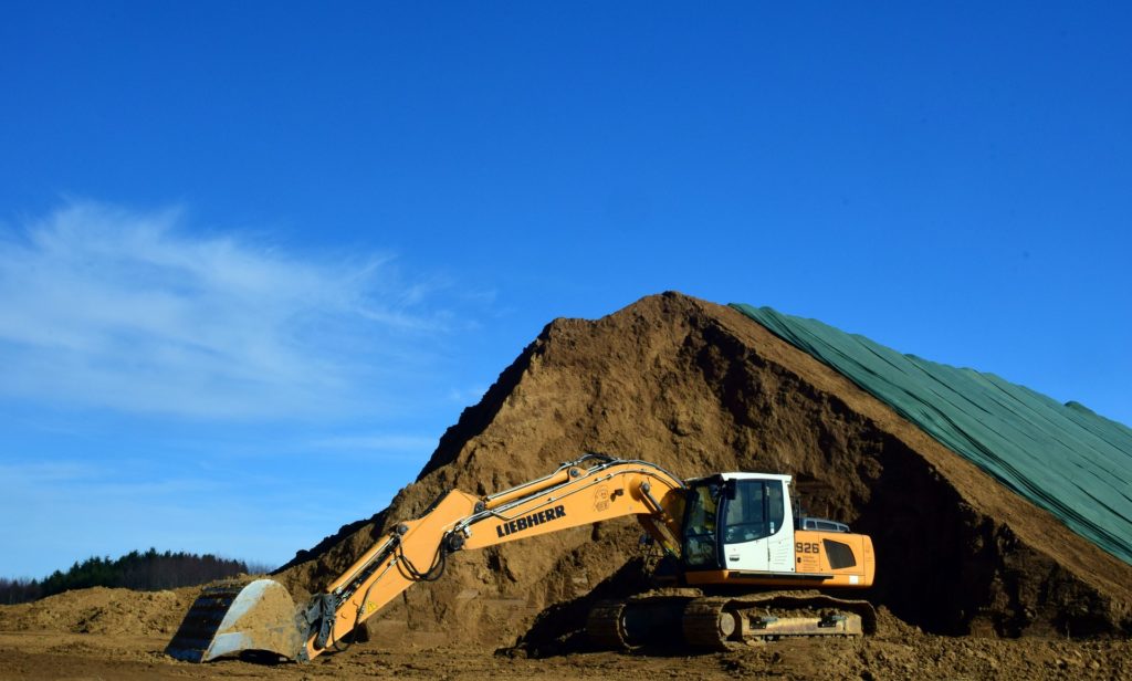Sometimes lower grade stockpiles are built up by the mine each year but only processed at the end of the mine life. Periodically the ore mining rate may exceed the processing rate and other times it may be less. This is where the stockpile provides its service, smoothing the ore delivery to the plant.

Scheduling can be done with variable time periods. Perhaps the schedule is generated using monthly time periods, or quarters, or years.

The 43-101 report will normally show the annual production schedule, but that does not mean it was generated that way. I prefer to use short time periods (monthly or quarterly) for the entire mine life, to ensure ore is always available to feed the plant. A 10 year mine life would result in 120 monthly time periods, so output spreadsheets can get large.

Scheduling can be done manually (in Excel) or by using commercial software, like Datamine’s NPVS. The commercial software is better in that it allows one to run different scenarios more quickly, and it does a lot of the thinking for the engineer. It also does a good job of stockpile tracking. It also decides when it is necessary to transition to mining in satellite pits.

Once the schedules are finalized, they are normally reviewed by the client for approval. The strip ratio and ore grade profile by date are of interest. One may then be asked to look to at different stockpiling approaches to see if an NPV (i.e. head grade) improvement is possible.

One can stockpile lower grade ore and feed the plant with better grade by mining at a higher rate with more equipment. One might need to examine iterative schedules of that type.

Sometimes one must take two steps backwards and re-design some of the initial pit phases to reduce waste stripping or improve grades. Then one would run the schedules again until getting one that satisfies everyone.

Now that the schedule is complete, we can write up the Chapter 16 text up to page 15. We’re getting closer to the end.

5. Site Layout Design

With the pit tonnages and mining sequence from the schedule, the mine engineers can start to look at the site layout (waste dumps and haul roads). Normally the tailings engineers will be responsible for the tailings layout. However, if there is no tailings engineer on the PEA team, the mining engineer may look after this too.

First there is a need for a waste balance. This defines how much mined overburden or waste rock will be needed to build haulroads, laydown pads, and tailings dams. Then the remaining waste volume must be placed into waste dumps.

Hopefully the tailings engineers have finished their tailings dam construction sequence by this time to provide their rockfill needs (although unlikely if you only gave them the production schedule two days ago).

The geotechnical engineers will provide the waste dump design criteria; for example, 3:1 overall side slope using 15m high dump lifts. Ideally it is nice to have soil and foundation information beneath the waste dump sites, but at PEA stage most often this isn’t available. The dump locations are only being defined now.

The mining engineers will size the various waste dumps to their required capacity. Then they can lay out the mine haulroads from the pit ramps exits to the ore crusher, the ore stockpiles, and to each waste dump.

That’s it for the site layout input. Add another 2 pages to Chapter 16. Now the mining engineers can look at the mining equipment fleet.

6. Fleet Sizing and Mining Manpower

The last task for the mine engineer in Chapter 16 is estimating the open pit equipment fleet and manpower needs. The capital and operating costs for the mining operation will also be calculated as part of this work, but the costs are only presented in Chapter 21.

The primary pieces of equipment are the haul trucks. They can range in size from 30 tonnes to 350 tonnes and anywhere in between.

Typically, the larger the equipment is, the lower the unit cost ($/t), especially in jurisdictions where labor costs are high. One doesn’t want a mine fleet with only 5 trucks nor one with 50 trucks. So where is the happy medium?

Once the schedule and site layout are complete, the mine engineers can run the truck haul cycles, in minutes. They need to estimate the time to drive from the pit face, up the ramp, to the waste dump, to the ore crusher, and return back into the mine. Cycle times determine the truck productivity, in tonnes per hour per truck and include the time to load the truck. Some destinations may have long cycle times (to a far off crusher) while others may be quick (to an adjacent waste dump).

The cycle time must be calculated for each material type going to each destination. As the pit deepens, the cycle times increase.

Very simplistically, if a 100 tonne truck has a 20 minute cycle time, it can do three cycles in an hour (300 tph). If one has to mine 10 million tonnes of ore per year, then that would require 33,300 truck hours. If a single truck provides 6500 operating hours per year, that activity would require a fleet of 5 trucks. The same calculation goes for waste.

The total trucking hours will vary year to year as waste stripping tonnages change or haul cycle times increase in deeper pits. The required truck fleet may vary year to year. Keeping haul distance short and haul cycles quick is the key to a lower cost mine.

The mine engineers undertake the productivity calculations for loading equipment to estimate annual operating hours, and the required shovel / loader fleet size.

The support equipment needs (dozers, graders, pickups, mechanics trucks, etc.) are typically fixed. For example, 2 graders per year regardless if the annual tonnages mined fluctuate.

The support equipment needs are normally based on the mining engineer’s experience. Hence the benefit of actually working at a mine at some point in your career.

Blasting includes both the blasthole drilling activity and hole charging. The mining engineer estimates drill productivity and specifications based on the bench height, the expected rock mass quality, and the power factor (kg/t) need to properly demolish the rock.

Finally, the mine operation manpower is estimated based on all the equipment operating hours as well as the fixed number of personnel to support and supervise the mine.

This essentially concludes the mining information presented in Chapter 16 of a typical 43-101 open pit report.

Conclusion

These two blog posts hopefully give an overview of some of the things that mining engineers do as part of their jobs. Hopefully the posts also shed light on the amount of work that goes into Chapter 16 of a 43-101 report. While that chapter may not seem that long compared to some of the others, a lot of the effort is behind the scenes.

Some will say PEA’s are not very accurate documents that should be taken with a grain of salt. One should understand that engineers are working with a limited amount of information at this early stage while forming the concept for the proposed operation.

The subsequent study stages are where more accurate costs are expected and can be demanded.

I don’t know if this overview makes one want to sign up to be a mining engineer or learn to code instead. None of this is rocket science; it just requires practical thinking.

If young people want to get into mining, but not sure into which aspect, I suggest go read through a 43-101 report. There are sections describing exploration, resource modelling, mine engineering, metallurgy, geotechnical engineering, environmental, and financial modelling. Its all in one document. See if any of these areas are of interest to you. Universities should use 43-101 reports as part of their mining engineering curriculum.

Note: You can sign up for the KJK mailing list to get notified when new blogs are posted. Follow me on Twitter at @KJKLtd for updates and other mining posts. The entire blog post library can be found at https://kuchling.com/library/

The Anatomy of 43-101 Chapter 16 – Mining (Part 1)

Date: March 20, 2024 Author: Ken Kuchling Comments: 4 Replies

When people learn that I’m a mining engineer, I’ll normally get perplexed looks and asked what that job is about. Most never even knew the job existed.

So I thought what better way to explain the mining engineer role than by describing the anatomy of a typical Chapter 16 (MINING) in a 43-101 Technical Report. That chapter is a good example of the range of tasks typically undertaken by mining engineers.

Secondarily it also provides an opportunity to describe in detail all the steps that go into writing a Chapter 16, focusing on the PEA.

PEA’s tend to have a poor reputation for lack of accuracy, and this blog post may shed some light on why that is. To avoid running on too long, I have subdivided this into Part 1 and Part 2.

Generally, one will see a single QP sign off on Chapter 16. However, the chapter requires input from several people. Section 16 is generally prepared in the same way for a PEA or a feasibility study (FS). The main difference is related to the amount of hard supporting data in a FS versus a PEA.

The PEA will rely on many “reasonable assumptions” and it can be done in at least half the time of a FS. A FS will also build on previous study decisions, something a PEA doesn’t have access to since it is a first time snapshot of a project.

Normally preparing Chapter 16 is done under time pressure to deliver results as quickly as possible. Other study team members are waiting for its output to finalize their own engineering work.

1. Define the Mine

In a PEA, the first thing that must be conceptualized is whether this will be an open pit (OP) mine, underground (UG), or a combination of both.

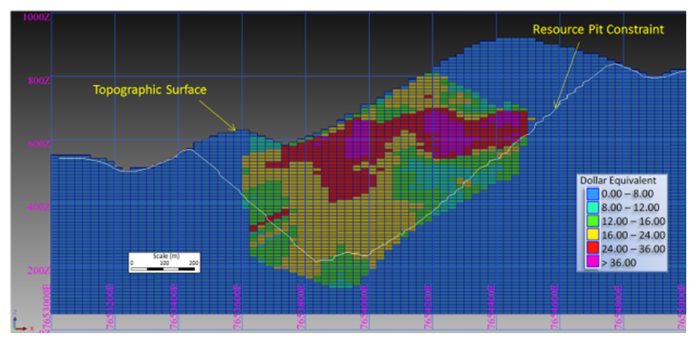There is always a mineral resource estimate available before doing a PEA. The way the resource is reported will indicate what type of mine this likely is. The geologists have already done some of the mining engineer’s work.

The mineral resource will suggest if this will be an OP or UG, a large or small operation, a long life or short life, and the likely processing method. The framework for the project is already set at the mineral resource estimate stage.

We can now write page 1 of Chapter 16.

2. Optimize the Pit Size and Shape

The first step for the mining engineer is a pit optimization analysis to define the approximate size and shape of the pit. The pit optimization step creates a series of nested economic pit shells for different metal prices. For example, the base case gold price may be $1800/oz, but we still want to see what size of pit would be economic at $1000/oz, $1200, $1300, etc. Normally one may run 50 different price scenario increments. The smaller shells may eventually be good starter pits to help improve NPV and payback time.

Before starting pit optimization, we require economic inputs from several people. The base case metal prices must be selected (normally with input from the client). The mining operating cost per tonne must be estimated (by the mining engineer). The processing engineers will provide the processing cost and recovery for each ore type.

The geotechnical engineers will provide approximate pit wall angles. All of these inputs have to be forecasted at a very early stage. We don’t yet know the size of the pit, the ore tonnage available, nor the actual plant throughput rate but one must still predict some costs. Hence these initial inputs might just be ballpark data.

In the final cashflow model you may eventually see slightly different metal prices, costs, or recoveries than used in pit optimization. That’s because that cashflow model inputs are generated by the study, while the optimization inputs are pre-study estimates.

The pit optimization step may also need to apply constraint boundaries. For example, if there is a nearby property limit or river, one may want to constrain the pit optimization to get no closer than 50 metres to the river or boundary. The pit shell optimizer may be free to expand the pit outwards in multiple directions, except that one direction.

Once the optimization is run, a series of nested pit shells are created, each with its own tonnes and grade. These shells are compared for incremental strip ratio, incremental head grade, total tonnes, and contained metal.

A decision must now be made on which shell to use for the mine design. Larger economic shells may have more tonnes, lower grade, and higher strip ratio. Smaller shells may have lower strip ratio and better grade.

For example, a smaller shell may have 10 year life containing 800,000 oz at a strip ratio of 2:1 while a larger shell may have 14 years, 1 million oz at a strip ratio of 3:1. Both are roughly the same economically. However, developing the larger shell may require more mining equipment capital yet have a lower average cost per tonne. Which shell do you choose?

There can be dozens of such shell to shell trade-offs and typically one doesn’t run schedules and cost models on all of them. The client will have input on whether they wish to move forward with 10 years 800,000 oz or the 14 years with 1 million oz. Sometimes selection is driven by investors having size expectations that need to be met.

Some people may say ‘Well… just run cashflow models for each case to see which is best”. The problem with doing too much analysis at this stage is that if you re-do the pit optimization with different recovery, operating costs, pit wall angles, you will get a different optimization result. It becomes a question of how much detail work to do on something that is based on very preliminary input parameters.

Assuming the mining engineers have now selected the preferred shell for mine design, they can move on to mine design. We can now write more of Chapter 16 to page 5.

3. Open Pit Design.

The mining engineer is now ready to undertake the pit design. The pit design step introduces a benched slope profile, smooths out the pit shape, and adds haulroads. Hence a couple of key input parameters are required at this time. The mining engineer will need to know the geotechnical pit slope criteria and the truck size & haul road widths. Let’s look at both of these.

Pit Slopes: Geotechnical engineers are responsible for providing the slope angle criteria to the mining engineers. The geotech engineers may have a lot or little information to work with. Perhaps they have geotechnical oriented core holes and they have undertaken some rock strength testing.

Perhaps the only information for the geotechnical engineers is rock quality data from exploration drilling. I have seen both situations at the PEA stage; the latter is more typical. In the feasibility study they would have geotechnical core hole data available. At the PEA stage, that is less likely, since no one yet knows the size and depth of the pit. We are only getting to that now.

Pit wall schematic

The geotechnical engineers will provide the inter-ramp slope angles, specified by catch bench widths and bench face angles. The engineers may subdivide slopes by rock type.

For example: the overburden wall is to be at 30 degrees, the underlying oxide rock at 40 degrees and the deeper fresh rock wall at 55 degrees. Additionally, the pit may be subdivided into pie shaped sectors, with differing slope criteria.

For example, the fresh rock on the west wall might have a 55 degree angle, but the east wall fresh rock may only allow 50 degrees and the south wall is 45 deg.

The more sectors and differing slope criteria, the more complex it is to do the pit design. Normally you don’t see geotechnical engineers signing off as QP’s for Chapter 16, although they had key input into the pit design.

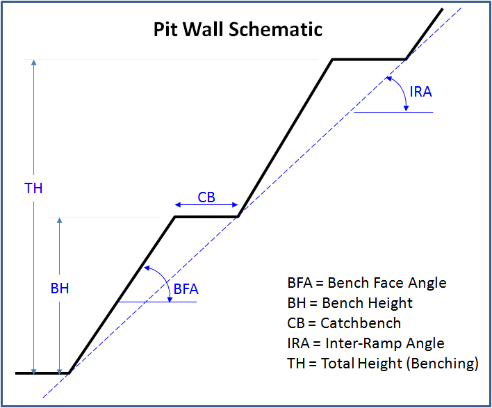
Ramps: Next the mining engineer needs to select the truck size, even though the production schedule has not yet been created.

Trucks sizes can vary between 30t up to 350t. A double lane ramp width is approximately 4.5 times the truck width, including space for a ditch and an outer safety berm. A 90 tonne truck is 6.7 metres wide (haulroad of 30m) while a 350 tonne truck is 9.8 m wide (haulroad of 44 m wide). That’s a 14m width difference.

The haul road gradient is normally 10%, which means a 200 metre deep pit requires a ramp length of 2000 metres to get to the bottom. It can be difficult to fit a 2 kilometre ramp in a small pit without pushing the walls out to provide enough circumference to get to depth.

Ramps can spiral around the pit, or they can zigzag back and forth on one side of the pit (switchbacks). The mine engineer will decide this once they see the topography, pit size, and ore body orientation. Adding ramps in a pit design pushes the crest outwards and adds waste to be stripped.

Pit Phases: After the pit design is complete, the mine engineer will design multiple interior phases to distribute the waste and ore tonnages in the mining schedule. These phases are sometimes referred to as pushbacks, laybacks, or stages. At mine start-up, one doesn’t want to strip the entire top off of a large pit. A smaller pit within the large pit will allow faster access to ore.

This completes the open pit design and now allows one to write to page 10 of Chapter 16. However, the mining engineer is not done yet.

Conclusion

This ends Part 1. In Part 2 we will discuss the mining engineer’s next tasks; production scheduling; waste dump design; and equipment selection. The mining engineer QP will sign off and take responsibility for all the mine design work done so far. You can read Part 2 at this link “The Anatomy of 43-101 Chapter 16 – Mining (Part 2)“.

Note: You can sign up for the KJK mailing list to get notified when new blogs are posted. Follow me on Twitter at @KJKLtd for updates and other mining posts. The entire blog post library can be found at https://kuchling.com/library/

Mine Builders vs Mine Vendors

Date: October 15, 2023 Author: Ken Kuchling Comments: Leave a reply

Normally when Major or Intermediate miners advance their projects through the study stages, they usually have the intent to build the mine at some time. Sometimes they may decide to sell the project if it no longer fits in their corporate vision or if they desperately need some cash. However, selling the project was likely not their initial intent.

On the other hand, Junior miners tend to follow one of two paths. They are either on (a) the Mine Builder path, or (b) the Mine Vendor path (i.e. sell the project). In this article, I will present some examples of companies on each path. There will also be some discussion on whether the engineers undertaking the early stage studies (e.g., PEA’s) should be considering the path being followed.

The Mine Builder Path

The Mine Builder generally follows a systematic approach, as sketched out in the image below. The project advances from drilling to Mineral Resource Estimate (MRE), scoping study (PEA), then through the Pre-Feasibility Study (PFS) and/or Feasibility Study (FS) stages. Environmental permitting is normally proceeding in conjunction with the engineering. Once the FS is complete, the next hurdles for the Mine Builder are financing and construction. The path is fairly orderly.

The amount of the exploration drilling is only needed to define an economic resource to the Measured and Indicated classifications. There is no requirement to delineate the mineral resource on the entire property since there will be time to do that during production. Demonstrating an economic resource, with some upside potential, is often sufficient for the Mine Builder.

Three examples of companies on the Builder path are shown below; Orla Camino Rojo gold project (in operation), SilverCrest Las Chispas gold project (in operation), and Nexgen Rook uranium project (financing stage). Although the duration of each timeline is different due to different project complexities, the development paths are consistent. Most junior miners would not consider themselves on the Builder path.

The Mine Vendor Path

Mine Vendor type organizations have the primary goal of selling their project. These companies may consist of management teams that don’t have the desire, comfort, or capability to put a mine into production. For example, this is often the case with companies founded by exploration geologists, whereby their plan is to explore, grow, and sell all (or part) of the project. In other cases the Junior miner realizes their project is large with a high capital cost. That capital cost is beyond the financial capability of the company. Hence a deep-pocket partner is required or an outright sale is preferred.

The Mine Vendors tend to follow a different development path than the Mine Builders. They don’t have the same long term objectives. Vendors want out at some point.

The Vendor path can be more irregular, with multiple studies undertaken at different levels of detail, sometimes stepping back to lower level of studies as more information is acquired. Their object is to make the project look good to potential buyers, and look better than their junior miner competitors also for sale. Often this ongoing project improvement process is termed “de-risking”.

Not only must the Vendors demonstrate an economic resource, they must demonstrate a highly valuable resource to maximize the acquisition price for the shareholders. They will try to do this through multiple drill campaigns followed by multiple studies, each one looking better than the prior one.

Sometimes you will see a management team indicate that, if the project isn’t sold, they are going to put it into production themselves. This may be true in some cases, or simply part of the negotiating game to try to maximize the acquisition price.

Two quick examples of companies on the Vendor path are shown below: Western Copper Casino project and Seabridge KSM project. The durations of these development timelines are extensive and expensive, while waiting for an interested buyer. During these periods, the companies may continue to spend money de-risk the project further. The hope is that the company can eventually make the project attractive or that changing market conditions will make it attractive for them. Unfortunately, there is always the possibility that no buyer will ever come along.

Engineer’s Perspective

One question is whether the independent geologists and engineers working on the advanced studies should be aware of the path the company is following. Is the company a Builder or a Vendor?

Some may feel that the technical work should be independent of the path being followed. Based on my experience as both an owner’s representative and independent study QP, I have a somewhat different opinion. The technical work should be tailored to the intended path.

The Engineer on the Mine Builder Path:

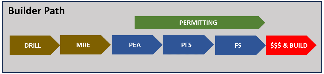
If an engineer understands that a Mine Builder’s project will move from PEA to PFS to FS in rapid succession, then there is more incentive to ensure each study is somewhat integrated.

For example, a PEA will use Inferred resources in the economics. However, if the project will advance to the PFS stage, where Inferred cannot be used, then it is important for the PEA to understand the role that Inferred plays in the economics. How much drilling will be needed to upgrade Inferred resource to Indicated for the PFS, if needed at all?

Typically, capital costs tend to increase as advancing studies get more accurate due to greater levels of engineering. A Builder wants to avoid large cost increases when moving from PEA to PFS to FS. Therefore, when costing at the PEA stage, one may wish to increase contingency or use conservative design assumptions. After all, one is not trying to sell or promote the project internally, but rather move it towards production.

There is no value to the Mine Builder by fooling themselves with low-balled cost estimates. (Although some may argue there is still a desire to low ball costs to get management to approve the project). Conversely Mine Vendors do have some incentive to low ball the costs.

Perhaps some of the recent project capital cost over-runs we have seen is that the Vendor mentality was used at the PEA stage to optimistically set the capital cost baseline. Subsequent studies were then forced to conform to that initial baseline. Ultimately construction will be the arbiter on the true project cost. Hence there is no real value in underestimating costs, ultimately making management appear incompetent if costs do over-run.

The Mine Builder will also be advancing environmental permitting simultaneously with their advanced studies. Hence at the early stage (PEA) it is important to properly define the site layout, processing method, production rate, facility locations, etc. since they all feed into the permitting documents.

Changing significant design details in the future will set back the permitting and construction timelines. Hence, for the Mine Builder, the engineers should focus on getting the design criteria mostly correct at the PEA stage. For the Mine Vendor, this is not as important since multiple studies are being planned for in the future anyway.

The Engineer on the Mine Vendor Path:

The objective of the Mine Vendor is to make the project attractive to potential buyers. There is less urgency in fast tracking detailed engineering and permitting.

It is not uncommon to see multiple drilling programs, followed my multiple studies of scenarios with different size, production rate, and layout. The degree of engineering conservativeness in design and costing is less critical since future studies may be on substantially different sized projects.

The role that the Inferred resource plays in the economics is also less important at this time, since a lot more drilling may be coming. The Vendor’s objective tends to be on maximizing resource size not necessarily optimizing resource classification.

While the Mine Vendor may also be advancing environmental permitting as another way to de-risk the project, the project design may still be in flux as the resource size changes. Major modifications to the plan may cause permitting to stop and re-start, leading to an extended project timeline and wasted money.

There is also risk in starting the permitting with a project definition that isn’t of economic interest to future buyers. Sometimes the Vendor may be making regulatory commitments that constrain the operating flexibility of future mine operators. Its easy to commit to things when you aren’t the one having to live up to them.

The Mine Vendor will also de-risk the project by moving from PEA to PFS and even to FS. The caution with completing a FS is that it is a costly study and essentially brings one to the end of the study line. What does the company do next if there is still no buyer?

Feasibility studies also have a shelf life, with the cost estimates and economics becoming inaccurate after a few years. Some companies may re-examine the project, re-frame it, and jump back to the PEA or PFS stages. There can be an on-going study loop, requiring continued funding with no guarantee of a sale in sight. Often feasibility studies have the dual role of trying to boost the share price and market cap, as well as frame the project for potential buyers.

Conclusion

As an engineer, it is helpful to understand the objectives of the project owner and then tailor the technical studies to meet those objectives. This does not mean low balling costs to make the study a promotional tool. It means focusing on what is important. It means recognizing the path, and what doesn’t need to be engineered in detail at this time. This may save the client time, money, and improve credibility in the long run.

In many cases, the precise size of the deposit is less important than understanding the site, access, water supply, local community issues, the environmentally acceptable location for dumps and tailings, etc.. It can be more important to focus on these issues rather than having a detailed mine plan with multiple pit phases that immediately becomes obsolete in a few months after the next drilling campaign.

Potential buyers will have their own technical team that will develop their own opinions on what the project should be and what it should cost. Just because a Mine Vendor has a feasibility study in hand, doesn’t mean a potential buyer will believe it.

This post is just a brief discussion of mining project timelines. For those interested, there a few additional project timelines for curiosity purposes. Each path is unique because no two mining projects are the same. You can find these examples at this link “Mining Project Timelines”.

Let me know about other interesting projects that have interesting paths to learn from. I can add them to the list.

Note: You can sign up for the KJK mailing list to get notified when new blogs are posted. Follow me on Twitter at @KJKLtd for updates and other mining posts. The entire blog post library can be found at https://kuchling.com/library/

Pit Optimization – More Than Just a “NPV vs RF” Graph

Date: October 14, 2021 Author: Ken Kuchling Comments: 3 Replies

In this blog I wish to discuss some personal approaches used for interpreting pit optimization data. I’m not going to detail the basics of pit optimization, assuming the reader is already familiar with it .

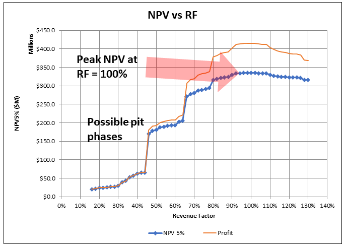Often in 43-101 technical reports, when it comes to pit optimization, one is presented with the basic “NPV vs Revenue Factor (RF)” curve. That’s it.

Revenue Factor represents the percent of the base case metal price(s) used to optimize for the pit. For example, if the base case gold price is $1600/oz (100% RF), then the 80% RF is $1280/oz.

The pit shell used for pit design is often selected based on the NPV vs RF curve, with a brief explanation of why the specific shell was selected. Typically it’s the 100% RF shell or something near the top of the NPV curve.

However the pit optimization algorithm generates more data than just shown in the NPV graph. An example of that data is shown in the table below. For each Revenue Factor increment, the data for ore and waste tonnes is typically provided, along with strip ratio, NPV, Profit, Mining cost, Processing, and Total Cost at a minimum.

Luckily it is quick and easy to examine more of the data than just the NPV curve.

In many 43-101 reports, limited optimization analysis is presented. Perhaps the engineers did drill down deeper into the data and only included the NPV graph in the report for simplicity purposes. I have sometimes done this to avoid creating five pages of text on pit optimization alone, which few may have interest in. However, in due diligence data rooms I have also seen many optimization summary files with very limited interpretation of the optimization data.

Pit optimization is a approximation process, as I outlined in a prior post titled “Pit Optimization–How I View It”. It is just a guide for pit design. One must not view it as a final and definitive answer to what is the best pit over the life of mine since optimization looks far into the future based on current information, .

The pit optimization analysis does yield a fair bit of information about the ore body configuration, the vertical grade distribution, and addresses how all of that impacts on the pit size. Therefore I normally examine a few other plots that help shed light on the economics of the orebody. Each orebody is different and can behave differently in optimization. While pit averages are useful, it is crucial to examine the incremental economic impacts between the Revenue Factor shells.

What Else Can We Look At?

The following charts illustrate the types of information that can be examined with the optimization data. Some of these relate to ore and waste tonnage. Some relate to mining costs. Incremental strip ratios, especially in high grade deposits, can be such that open pit mining costs (per tonne of ore) approach or exceed the costs of underground mining. Other charts relate to incremental NPV or Profit per tonne per Revenue Factor. (Apologies if the chart layout below appears odd…responsive web pages can behave oddly on different devices).

Conclusion

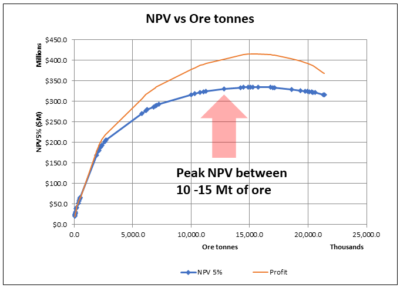
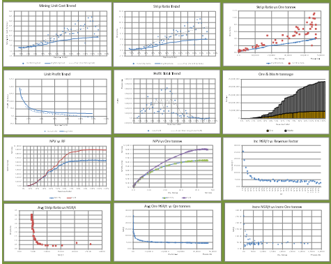It’s always a good idea to drill down deeper into the optimization output data, even if you don’t intend to present that analysis in a final report. It will help develop an understanding of the nature of the orebody.

It shows how changes in certain parameters can impact on a pit size and whether those impacts are significant or insignificant. It shows if economics are becoming very marginal at depth. You have the data, so use it.

This discussion presents my views about optimization and what things I tend to look at. I’m always learning so feel free to share ways that you use your optimization analysis to help in your pit design decision making process.

As referred to earlier, there is a lot of uncertainty in the input parameters used in open pit optimization. These might include costs, recoveries, slope angles and other factors. If you would like to read more, the link to that post is here. “Pit Optimization–How I View It”.

Note: You can sign up for the KJK mailing list to get notified when new blogs are posted. Follow me on Twitter at @KJKLtd for updates.

Heap Leach or CIL or Maybe Both

Date: July 14, 2020 Author: Ken Kuchling Comments: 1 Reply

Typically gold mines consist of either a heap leach (HL) operation or a CIL type plant. There are a few projects that operate (or are considering) concurrent heap leach and CIL operations. Ultimately the mineral resource distribution determines if it makes economic sense to have both. This blog discusses this concept based on past experience.

A CIL operation has higher capital and operating costs than a heap leach. However that higher cost is offset by achieving improved gold recovery, perhaps 20-30% higher. At higher gold prices or head grades, the economic benefit from improved CIL recovery can exceed the additional cost incurred to achieve that recovery.

Some background

Several years ago I was VP Engineering for a Vancouver based junior miner (Oromin Expl) who had a gold project in Senegal. We were in the doldrums of Stage 3 of the Lassonde Curve (read this blog to learn what I mean) having completed our advanced studies. Our timeline was as follows.

Initially in August 2009 we completed a Pre-Feasibility Study for a standalone CIL operation. Subsequently in June 2010 we completed a Feasibility Study. The technical aspects of Stage 2 were done and we were entering Stage 3. Now what do we do? Build or wait for a sale?

The property’s next door neighbor was the Teranga Sabodala operation. It made sense for Teranga to acquire our project to increase their long term reserves. It also made sense for a third party to acquire both of us. The Feasibility Study also made the economic case to go it alone and build a mine.

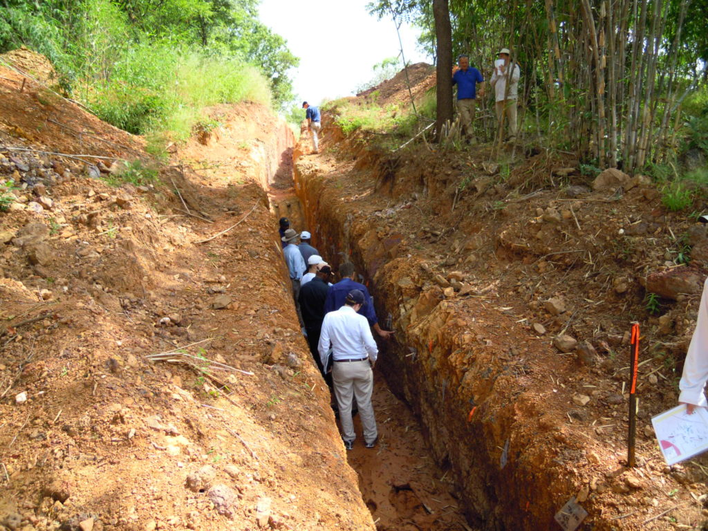While waiting for various third-party due diligences to be completed, the company continue to do exploration drilling. There were still a lot of untested showings on the property and geologists need to stay busy.

Two years later in 2013 we completed an update to the CIL Feasibility Study based on an updated resource model. Concurrently our geologists had identified seven lower grade deposits that were not considered in the Feasibility Study.

These deposits had gold grades in the range of 0.5 to 0.7 g/t compared to 2.0 g/t for the deposits in the CIL Feasibility Study. We therefore decided to also complete a Heap Leach PEA in 2013, looking solely on the lower grade deposits.

These HL deposits were 2-8 km from the proposed CIL plant so their ore could be shipped to the CIL plant if it made economic sense. Test work had indicated that heap leach recoveries could be in the range of 70% versus >90% with a CIL circuit. The gold price at that time was about $ 1,100/oz.

Ultimately our project was acquired by Teranga in the middle of 2013.

Where should the ore go?

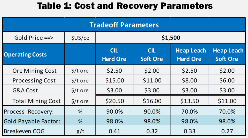With regards to the Heap Leach PEA, we did not wish to complicate the Feasibility Study by adding a new feed supply to that plant from mixed CIL/HL pits. The heap leach project was therefore considered as a separate satellite operation.

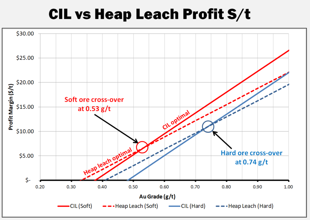The assumption was that all of the low grade pit ore would go only to the heap leach facility. However, in the back of our minds we knew that perhaps higher grade portions of those deposits might warrant trucking to the CIL plant.

For internal purposes, we started to look at some destination trade-off analyses. We considered both hard (fresh rock) and soft ore (saprolite) separately. CIL operating costs associated with soft ore would be lower than for hard ore. Blasting wasn’t required and less grinding energy is needed. The CIL plant throughput rate could be 30-50% higher with soft ore than with hard ore, depending on the blend.

I have updated and simplified the trade-off analysis for this blog. Table 1 provides the costs and recoveries used herein, including increasing the gold price to $1500/oz.

The graph shows the profit per tonne for CIL versus HL processing methods for different head grades.

The cross-over point is the head grade where profit is better for CIL than Heap Leach. For soft ore, this cross-over point is 0.53 g/t. For hard ore, this cross over point is at 0.74 g/t.

The cross-over point will be contingent on the gold price used, so a series of sensitivity analyses were run.

The typical result, for hard ore, is shown in Table 2. As the gold price increases, the HL to CIL cross-over grade decreases.

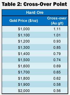These cross-over points described in Table 2 are relevant only for the costs shown in Table 1 and will be different for each project.

Conclusion

It may make sense for some deposits to have both CIL and heap leach facilities. However one should first examine the trade-off for the CIL versus HL to determine the cross-over points.

Then confirm the size of the heap leach tonnage below that cross-over point. Don’t automatically assume that all lower grade ore is optimal for the heap leach.

If some of the lower grade deposits are further away from the CIL plant, the extra haul distance costs will tend to raise their cross-over point. Hence each satellite pit would have its own unique cross-over criteria and should be examined individually.

Since Teranga complete the takeover in mid 2013, we were never able to pursue these trade-offs any further.

Note: You can sign up for the KJK mailing list to get notified when new blogs are posted. Follow me on Twitter at @KJKLtd for updates and insights.

Connecting With Investors – Any New Ideas?

Date: April 2, 2020 Author: Ken Kuchling Comments: Leave a reply

I recently read some LinkedIn posts from junior mining executives and IR staff asking for ideas about new ways to engage with investors. The commonly used ways rely on PowerPoints, webinars, and trade show booths. However during this Covid-19 crisis, trade shows are no longer an option. Therefore these face to face discussions with investors will now be missing. This will impact on the ability of a company to connect with and establish trust with those people.

What else can be done?

Perhaps with technology, like Zoom, one can replicate the personal feel of a trade show booth. One can still have back and forth conversations with investors rather than just doing lecture style webinars.

Free discussion is good in most cases. Letting investors feel they are sitting around a table will give them a better understanding of how management thinks and how decisions are being made. It will also help them get to know the personality of the management team.

I’m not an IR person but I admire the job they have to do, especially in today’s business environment. I have recently sat in on several junior mining online webinars. When listening to the Q&A’s afterwards, it is apparent that many attendees enjoyed understanding the technical aspects of a project. However they will only get that understanding by asking questions. Trade show booths gave them that opportunity.

Technology gives some options. Like what?

Set up regularly scheduled Zoom meetings, enabling investors to have interactive back and forth conversations with management. Try to avoid long presentations with questions only at the end. Have a moderator review and ask questions as they come in.

Management teams should introduce more than just the CEO or COO. Include VP’s of geology, engineering, corporate development, from time to time. Don’t hesitate to let the public meet more of your team. Trade show booths are often manned by different team members.

Pick different topics for discussion on each conference call to avoid repeating the same PowerPoint over and over again.

Avoid being too scripted.

For example one call could be a fly-around of the property using Google Earth. Another call could focus on the ore body and resource model. Another call might discuss metallurgy and the thought process behind the flow sheet. Perhaps discuss the development options you have considered.

None of this information is likely confidential if it has been presented in your 43-101 report.

Companies file highly technical 43-101 reports on SEDAR, but then let the investors fend for themselves. One could take some online time for high level walk through of the report. Clearly explain technical issues and how they have been addressed or will be addressed in the future. This is an opportunity to explain things in plain English, and field questions.

One downside to such calls is if there are significant flaws with a project. Open discussions may help expose them. One needs to know your own project well, be aware of all the issues, and have them under control in one way or another.

Conclusion

Better communication with investors can increase confidence in a management team. Although some investors may not enjoy technical discussions, I think there is a subset that will find them very helpful and interesting. There will likely be an audience out there.

Mining projects are complex with many moving parts and many uncertainties. Trust and confidence will come if a company is transparent in what they are doing and explain why they are doing it.

The mining industry is looking for new ways to reach out, so it shouldn’t be afraid to try new things. Some management teams will be great at it, others not so much. Figure out where you fit in.

Unfortunately one of the aspects of trade shows that cannot be replicated is the ability for investors to wander around aimlessly, take a quick glance at a lot of companies, and then decide which ones they want to learn more about.

Warning: zoom bombing

As an aside, if you are using Zoom make sure the host has configured the right settings. There are instances where anonymous participants can suddenly share their own computer screen, i.e. with questionable videos, to the group. It’s been referred to as “zoom bombing”.

https://www.forbes.com/sites/leemathews/2020/03/21/troll-terrifies-zoom-meeting-zoombombing/#2765abfc3e70

https://www.businessinsider.com/zoom-settings-change-avoids-trolls-porn-2020-3

Note: You can sign up for the KJK mailing list to get notified when new blogs are posted.

Follow me on twitter (@KJKLtd) or LinkedIn at https://www.linkedin.com/in/kenkuchling/)

Global Tax Regimes – How Do They Compare?

Date: February 9, 2016 Author: Ken Kuchling Comments: 3 Replies

Update: This blog was originally written in Feb 2016, but has been updated in Aug 2019.

As a reminder for all QP’s doing economic analysis for PEA’s, don’t forget that one needs to present the economic results on an after-tax basis.

Every once in a while I still see PEA technical reports issued with only pre-tax financials. That report is likely to get red- flagged by the securities regulators. The company will need to amend their press release and technical report to provide the after tax results. No harm done other than some red faces.

Taxes can be complicated

When doing a tax calculation in your model, where can you find international tax information? PWC has a very useful tax-related website. The weblink below was sent to me by one of my industry colleagues and I thought it would be good to share it.

The PWC micro-site provides a host of tax and royalty information for selected countries. The page is located at https://www.ey.com/gl/en/services/tax/global-tax-guide-archive

On the site they have a searchable database for tax information for specific countries.

The PWC tax and financial information includes topics such as:

Corporate tax rates
Excess profits taxes
Mineral taxes for different commodities
Mineral royalties
Rates of permissible amortization
VAT and other regulated payments
Export taxes
Withholding taxes
Fiscal stability agreements
Social contribution requirements

PWC has a great web site and hopefully they will keep the information up to date since tax changes happen constantly. The website also has a guide related to the rules for the treatment of capital expenditures. Check it out. https://www.ey.com/gl/en/services/tax/global-tax-guide-archive

Note: If you would like to get notified when new blogs are posted, then sign up on the KJK mailing list on the website. Otherwise I post notices on LinkedIn, so follow me at: https://www.linkedin.com/in/kenkuchling/.

There is a unique paradox sitting at the heart of how the mining industry evaluates its projects. It’s called the Inferred Resource—now you see it, now you don’t.

What Are Inferred Resources?

Inferred resources represent the lowest confidence category of mineral resources; typically estimated in zones with limited sampling and unconfirmed geological continuity. They carry the highest geological uncertainty of the three resource categories.

In Preliminary Economic Assessments (PEAs), Inferred resources are allowed—but only under certain conditions:

They can be included in mine plans and economic models, which is the reason PEAs exist: to allow early-stage projects to test economic viability using all available resource data.

Inferred tonnes are routinely used to extend mine life or improve project economics in PEA studies. Investors must understand this risk and should examine the proportion of mined tonnage that is classified as Inferred. This breakdown is normally presented in the Technical Report.

Conversely, in Pre-Feasibility Studies (PFS) and Feasibility Studies (FS), the rules for Inferred material are different:

Inferred resources cannot be included in mineral reserve estimates or in the economic analysis underpinning a PFS or FS. Inferred “ore” is treated as waste rock.

Only Indicated and Measured resources can be converted to Probable and Proven mineral reserves.

Including Inferred material in a PFS mine plan would typically disqualify the study from being used for project financing or a production decision.

Some companies might include Inferred material in a PFS as “upside” or as a sensitivity case, but that analysis must be clearly distinguished from the base case.

The resource upgrade requirement (from Inferred to Indicated) creates some interesting dynamics:

Companies will look at ways to compensate for the Inferred material deduction. Cutoff grade changes and step out drilling are ways to mitigate this impact.

A large Inferred resource that cannot be upgraded without great cost (due to depth, remoteness, or lack of ore-zone continuity) can permanently stall a project at the PEA stage. Hence, one may see multiple PEAs completed on the same project (i.e., the PEA loop).

In closing, the peculiarity of the Inferred resource is that it is essentially a tiered permission structure. Inferred resources are useful for early economic screening, but they must be converted to higher-confidence categories before they can support a bankable study or project debt financing.

Permitting via a PEA

Companies sometimes will commence the permitting process based on their PEA study. There are some risks to doing this, and the Inferred resource creates one of these risks.

Baseline studies for hydrology, ecology, and air quality typically require two to three years of data collection. So starting early makes sense, even with only a PEA-level project layout in hand.

Jurisdiction may play a role too. Some areas are more receptive to early-stage permitting engagement. Other permitting processes may be more rigorous such that operators want at least a PFS in hand before committing to a full EIA process.

How Can Inferred Resources Affect Permitting

Let us examine some specific aspects of permitting that can be influenced by Inferred resources.

(a) Permit the smaller FS footprint and risk under-permitting if Inferred is later upgraded. Requesting future permit modification for a suddenly larger project is sometimes viewed by regulators as “permitting by stealth”.

(b) Permit the larger PEA footprint to provide flexibility, which may trigger more extensive environmental review and higher bonding requirements.

2. Environmental Impact Assessment (EIA) Scope & Cost: A mine plan that includes Inferred material:

3. Tailings and Waste Facility Sizing: Tailings storage facilities (TSFs) and waste rock dumps are sized to the life-of-mine tonnage. Inferred tonnes included in a PEA can drive facility sizing significantly. Permitting a TSF for a larger tonnage is:

– More difficult and time-consuming to obtain if the height and footprint increase

– Will be subject to more rigorous dam safety and closure review- However this could be potentially beneficial if the Inferred resource is later confirmed during mining

4. Financial Assurance and Reclamation Bonding: Regulators require bonds or financial assurances sized to the cost of full site reclamation. A larger mine footprint driven by Inferred tonnes means:

– Higher bonding requirements

– Larger financial burden on the company during the project development phase

– Potential difficulty for junior companies in securing bonds for Inferred-inflated footprints that have not been proven out yet.

6. Indigenous and Community Consultation: In jurisdictions with consultation requirements (Canada’s duty to consult, FPIC principles, etc.), the scope of consultation is tied to the project’s impact footprint and duration. A mine life extended by Inferred tonnes:

– Triggers consultation over a longer operational period

– May affect benefit agreement negotiations (royalties, employment commitments) tied to mine life or total tonnage

– If mine life subsequently shrinks at FS stage, it can create credibility and trust issues with communities who were counting on a longer mine life.

In closing, personally I feel that project proponents should try to permit to a footprint somewhat larger than the Pre-Feasibility base case to preserve operation flexibility. For more on the benefits of flexibility, see the blog post “Mining’s Obsession with Optimization – Good or Bad”.

Conclusion

Inferred resources present a unique paradox; they can and can’t be used in mining economic analysis. They can be used to examine project viability but can’t be used to make a production decision.

The manner in which Inferred resources are viewed can also affect permitting. Although they don’t directly enter the regulatory process, they can shape the physical parameters of the mine plan that regulators will evaluate.

Even if a company grows the resource size between the PEA and PFS, there will still be a component of Inferred material within the PFS mine design that might be considered real tonnage or not.

Getting the permitted footprint right relative to the eventual resource confidence level is an underappreciated skill in project development. Each mining project is unique, and there is no easy one-size fits all solution when considering the impact of Inferred resources on project development.

In case you missed it, the last blog post was ” Mining’s Obsession with Optimization – Good or Bad“. https://kuchling.com/minings-obsession-with-optimization/ The entire blog post library can be found at https://kuchling.com/library/

You can sign up for the KJK mailing list to get notified when new blogs are posted. Follow me on LinkedIn or Twitter (@KJKLtd) for updates and other mining commentary.

Recently I’ve seen a few LinkedIn conversations about whether the mining industry is spending enough money on Research and Development (R&D). Usually when one thinks of R&D, one might envision the development of new technology, new drug, equipment or software.

This blog post examines whether the junior mining industry was a leader in Tech Startup culture. Even things like the Lassonde Curve and the PEA have their comparables in the current tech world.

Are Junior Miners precursors to Tech Startups

Junior mining companies and Tech Startups share numerous similarities, although they operate in very different worlds. The following comments should recognize that junior mining ecosystem has been around for generations, long before the birth of tech ecosystems.

A startup spends years (and millions of dollars) building an MVP (Minimum Viable Product). If the market doesn’t want it or the tech fails to scale, the company goes to zero. Similarly if holes don’t hit or the metallurgy is too complex, the mining asset can face significant headwinds.

Both generate proprietary data. A Junior Miner’s most valuable asset is often its geological data (drill results, resource estimates, land tenure). A Tech Startup’s asset is its IP, code, or trade secrets. In both cases, the assets are largely intangible until proven economic.

Both rely on quality founders and management. A small, skilled team can make or break the company. A geologist or executive with a great track record (“the Midas touch”) is analogous to a serial tech founder. Often the investors are backing the person more than the project.

Obviously we should also point out there some differences between juniors and Tech Startups.

Juniors work with physical geological reality. You either find the ore body or you don’t. Startups can pivot; geology can’t.

Mining has far longer timelines; discovery to production can take 10–20 years vs. a startup’s typical 5–7 year VC cycle. Any longer than that, and a Tech Startups technology can become obsolete.

Regulatory, environmental permitting, and social license is a constraint for miners with no real startup equivalent. Viable exploration projects can get blocked through no fault of the miner itself.

Junior Miners are more commodity-price dependent. Even a great deposit can be uneconomic at the wrong metal price. Conversely a miner’s asset could become more valuable over time based on metal prices. Tech startup do not rely on a commodity price outside their control.

The startup world will label their financing rounds (seed, Series A, Series B,..) with the hope that future investors provide financing at higher valuations than earlier investors. The mining industry does not label their placement rounds – perhaps they should.

In conclusion, an analogy between Junior Miners and Tech Startups can help outsiders understand the risk, capital structure, and investor behavior of both industries. One might conclude that Junior Miners were the Tech Startups of decades prior, and are still functioning that way today.

Should exploration expenses be considered R&D

Exploration spending shares some of the same characteristics of more commonly R&D.

R&D is about de-risking a concept, and de-risking is a term commonly used by Junior Miners. Every drill hole, soil sample, and geophysical survey is a data point that builds knowledge, and even uneconomic drill holes provide value by focusing the search area.

Much like our drug development example, exploration has a high-failure, high-reward path. Early-stage “lab work” (geochemistry/geophysics) leads to “clinical trials” (core drilling) and eventually “commercialization” (feasibility and production).

Exploration also tends to be more binary since it is geologically constrained. You either find an ore body or you don’t. You can’t modify or pivot with an orebody. On the other hand, drug and software R&D can yield partial successes or new technologies, that may have other applications.

Although there are both similarities and differences, the analogy is interesting. Exploration may be considered as a hybrid since it has the uncertainty and knowledge-creation aspect of R&D, but the result is a unique physical asset and not IP. In my view exploration is equivalent to R&D.

Lassonde Curve vs Hype Cycle Curve

As mentioned previously, junior mining and Tech Startups will follow a cyclic path of hype and despair. In mining it is known as the “Lassonde Curve” and in tech its called the “Gartner Hype Cycle”. Let’s look at the similarities. Which came first?

The Lassonde Curve is the “elder” of the two models, predating the Gartner Hype Cycle by about a decade. I had written a previous blog post on this at Mining’s Lassonde Curve – A Wild Ride.

Is a PEA Study Like a Tech Product Market Fit (PMF) Study

Another similarity between junior mining and tech world is in the way early-stage viability is assessed. This is required to decide whether millions of dollars of further investment is warranted. Miners will complete a PEA. Startups will complete Product-Market Fit research.

A Preliminary Economic Assessment (PEA or scoping study) is an early-stage technical and economic evaluation of a mineral deposit. Its core purpose is to determine whether a project is potentially viable before committing significant capital to more advanced studies.

Product-Market Fit (PMF) research for a Tech Startup is a structured effort to determine whether a product satisfies a strong market demand. The goal isn’t just to confirm PMF exists; its to understand the who, why, and how it will work before committing to aggressive growth.

1. The “Does This Thing Actually Work?” Test

– Tech (PMF): Once the team has built a beta, they can see if people are using it and are willing to pay for it. They need to prove there is a market for the tech.

– Mining (PEA): The team has found a deposit. The PEA is the first time they can put a dollar sign on it. It’s a conceptual study that predicts “If we build a mine here with these current economic inputs, it should make money.”

2. The Shift from “Geology” to “Economics”

Just as a Tech Startup shifts from coding to customer acquisition cost (CAC), a Junior Miner shifts from geology to metallurgy and CAPEX.

– Tech: It doesn’t matter how good the code is, if it costs >$50 to acquire a customer who only spends $5 it will not be a viable venture.

– Mining: It doesn’t matter if you have 2 million ounces of gold if the rock is difficult to process or if the project costs billions to build. The PEA is the first reality check on these costs.

3. Attracting the Investors

The PEA / PMF stage may be the ultimate gatekeeper for many institutional capitalists.

– Tech: Once you deliver a PMF, Venture Capital (VC) firms may be more willing to provide growth capital to scale the business.