
Have worked in the mining industry for over the last 40 years it is always interesting to watch the herd mentality that exists. Its obvious how easily the industry gets caught chasing the latest fads.
All it takes is a short term spike in a commodity price or a big discovery somewhere and then off we go running in that direction. It doesn’t matter the rationale driving the event, companies know they need to be in there and investors don’t want to miss out either. Its FOMO; the fear of missing out.
Don’t be the last on the bandwagon
In my experience, the fads or crazes can be based on commodities, locations, or technologies. The mining industry is very flexible in that regard. I’ll give a few examples that I have seen. You probably have even more from your own experience.
Commodity Fads
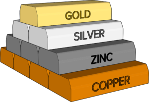 It seems that as soon as there is a price spike or positive market narrative, a commodity specific projects can take on a life of their own. The following list gives a few examples and, when you reflect upon them, ask how many actually came into successful production. These events occur at different times in different economic cycles.
-
Potash: a few years ago potash prices spiked and potash leases were all the fad no matter where they were located around the globe, be it Canada, Russia, Ethiopia, Thailand, Brazil, etc. That craze has largely fizzled out as prices returned to normal. But just wait for the next temporary price spike.
-
Lithium / Graphite: as soon as green battery technology started to be promoted in the news in 2016, miners couldn’t run fast enough to pick up the lithium properties. The same idea holds for battery metals such graphite, vanadium, cobalt, and also rare earth categories. After a lull, the process repeats itself in 2022.
-
Uranium: years ago uranium prices spiked and Ur properties were hot everywhere. Prices have dropped but seem to be ramping up in late 2018.
-
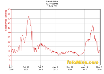
Cobalt Excitement Curve
Cobalt: see the price chart on the right to see how cobalt went into a craze and then out of it.
-
Nickel: years ago a spike in nickel prices caused a surge in nickel properties, whether it was sulphide nickel, laterite nickel, or other forms.
-
Iron Ore: in conjunction with the Chinese construction boom, iron ore properties were hot around the globe, in high cost or low cost jurisdictions, it didn’t matter where the property was. Iron is still being pursued but mega scale projects always overhang the market.
-
Diamonds: in conjunction with the first diamond discoveries in Canada in the 1990’s, diamond properties became hot, whether in the Canada or around the globe. If you couldn’t get a property in Canada’s NWT boom area, anywhere else globally was fine too.
-
China in general: a few years ago every base metal project was thought of as either a potential supplier to China or a potential acquisition for Chinese companies. As long as it could meet Chinese investor interest it was good.
Regional Exploration Fads
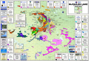 We have all seen the staking rushes that occur when a world class prospect is discovered. I’m sure we can all recall getting the large claim maps (as shown) with their multicolored graphics showing the patchwork of acquisitions around a discovery. PDAC was great for distributing these. They were well done and interesting to study.
Picking up properties in hot areas became the fad and share prices would move upwards regardless of whether there was any favorable geology on the property. Who recalls the following?
-
Voisey Bay: with a mad staking rush around there, with nothing else really paying off in the long run.
-
Saskatchewan: the potash staking rush where almost every inch of the potash zone was staked with only a couple of companies eventually moving forward and only one going into production.
-
Indonesia: during Bre-X people could not acquire properties in Indonesia fast enough.
-
NWT: where the diamond property staking rush was crazy in the mid 1990’s.
Technology Fads
 Even mining or processing technologies could get caught up in somewhat of a wave and become a fad for further study. Sometimes this is driven by suppliers or consultants. For the engineers out there, who can recall…
-
Paste Tailings: with numerous conferences and consultants promoting thickened or paste tailings technology as the panacea. This lead to numerous studies related to thickening, pumping, and disposal at each mine.
-
Block Caving: whereby in order to deliver high tonnages at low cost, bulk underground mining was being promoted. Everyone wanted their underground project to be a low cost caving style operation.
-
High Pressure Grinding Rolls (HPGR): where process consultants would highlight HPGR as the new replacement for conventional grinding mills. I’m not sure this technology has taken the industry by storm as they were hoping in the 1990’s.
-
IPCC: whereby inpit crushing and conveying systems were being promoted in many articles and global conferences as the solution to operating cost issues. I think implementation of IPCC technology isn’t as simple as envisioned and I’m not aware of many cases of its successful implementation.
-
Dot.com: in the early 2000’s many junior miners left exploration behind and transitioned to the dot.com boom, a fad that essentially went nowhere for most.
-
Pre-concentration: this seems to be a growing technology that may be gaining momentum. It isn’t new technology and it will definitely have its benefits. However a big stumbling block is how many deposits are actually suitable for its application. I have written more about this technology “Pre-Concentration – Savior or Not?“
Conclusion


 Their corporate website states that they would pay, for a specified period of time, the claim fees/taxes related to existing mineral properties or related to the staking of new mineral properties.
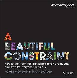
 The term Theory of Constraints may be common to some. However that concept is different than what is being discussed in the book. The TOC essentially relies on managing a constraint or eliminating it, and then addressing the next constraint in sequence.

 The tech start-up model is similar to the junior mining business model as it relates to early stage funding followed by additional financing rounds. One obvious difference is that mining mainly uses the public financing route (IPO’s) while the tech industry relies on private equity venture capital (VC’s).
 My first experience with the tech industry was associated with the many after-hours networking meetings called “meetups”. They are held weeknights from 6 to 9 pm and consist of guest speakers, expert panels, and for general networking purposes. Often guest speakers will describe their learnings in starting new companies and failures they had along the way.
 Most of the tech meetups are held in local tech offices. These offices are great. They have an open concept, pool tables, ping pong, video games, fully stocked kitchen. Who wouldn’t want to work there?
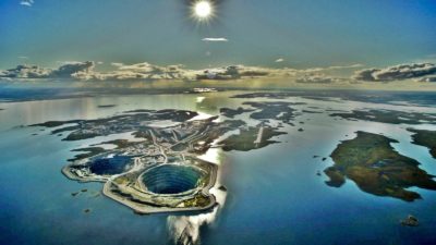 In the late 1990’s I was working in the Diavik engineering office in Calgary. They provided a unique office layout whereby everyone had an “office” but no front wall on the office so you couldn’t shut yourself in. There were numerous map layout tables scattered throughout the office to purposely foster discussion among the team.
 One specific example that I have seen is related to the 2015 disposition of foreign resource assets by both Barrick and Ivanhoe to Zijin, a Chinese company. I don’t know much about Zijin, other than having heard Norway’s government directed its $790 billion oil fund to sell holdings in some companies because of their environmental performance. Zijin was one of these companies.
 It will be interesting to see whether the idea of governments sanctioning the acceptability of acquirers in the mining industry will gain traction.
 Irrespective of 43-101, if you are working at a mining operation the last thing you want to do is present management with an incorrect reserve, pit design, or production plan.
 As a QP, I suggest the onus is on the software developers to demonstrate that they can produce reliable and comparable results under all conditions. They need to be able to convince the future users that their software is accurate.
 A failure cleanup fund

 So there likely is a significant network of experienced people out there. It’s just a matter of being able to tap into that network when someone needs specific expertise.
 Mining companies are constantly in the media with stories of cost over-runs, mine shutdowns, fatalities, strikes & protests, and environmental incidents.
 The larger mining companies will always have their investors like pension funds and mutual funds, however the junior miners may be a different story.