As a mining engineer, I am not usually called in to review a project that is still at the exploration stage. This is normally the domain of the geologist. However from time to time I have an interest in better understanding the potential of an early stage mining project. This could be on behalf of a client, for investing purposes, or just for personal curiosity.
 At the exploration stage one only has drill interval data from news releases to examine. A resource estimate may still be unavailable.
The drill data can consist of long intervals of low grade or short intervals of high grade and everything in between. What does it all mean and what can it tell you?
The following describes an approach I use for examining early stage gold deposits. The logic can be expanded to other metals but would take more effort.
My focus is on gold because it has been the predominant deposit of interest over the last few years, and it is simpler to analyze quickly.
We All Like Scatter Plots
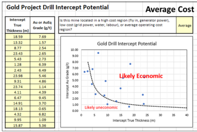
My approach relies on a scatter plot to visual examine the distribution of interval thicknesses and gold grades. Where these data points cluster or how they are distributed can provide some prediction on the overall economic potential of a project. Its not a guarantee, but only an indicator.
I try to group the analysis into potential open pit intervals (0 to 200 metres from surface) and potential underground (deeper than 200m) intervals. This is because a 20m wide interval grading 2.0 g/t is of economic interest when near surface, however of less interest if occurring at a 300m depth.
 Using information from a news release, I create a two column Excel table of highlighted intervals and assay grades. The nice thing about using intervals is that the company has provided their view of the mineable widths.
If one is provided with raw 1-metre assay data you would have to make that decision, which can be a significant task. The company has already helped make those decisions.
Normally I tend to use the highlighted sub-intervals and not the main intervals since issues with grade smoothing can occur.
A large interval containing multiple high grade sub-intervals may see some grade smoothing.This happens if the grade between sub-intervals is very low grade or even waste. It takes a fair bit of effort to assess this for each drill hole, hence it is easier to work with the sub-intervals.
I have an online calculator (Drill Intercept Calculator) that lets you assess if grade smoothing is occurring.
When inputting the interval thickness, I prefer to use the true thickness and not the interval length. If the assay information does not specify true thicknesses, then I simply multiple the interval length by 0.70 to try to accommodate some possible difference in width. Its all subjective.
The assays can consist of Au (g/t) or AuEq (g/t) if more metals are present. If very high grades are encountered (greater than 10 g/t) I simply input 9.9 g/t into the Excel table so they fit onto my scatter plot. Extremely high grades can be sporadic and localized anyhow.
Finally I need to decide whether the project is located in a region of high operating cost, low cost or about average costs. High costs could be with a fly in/ fly out, camp operation, with diesel power, and seasonal access.
A low cost operation could be in temperate climate, with good access to local infrastructure, water, labour, and grid power. An average operation would be somewhere in between the two. Its just a gut feel.
Results
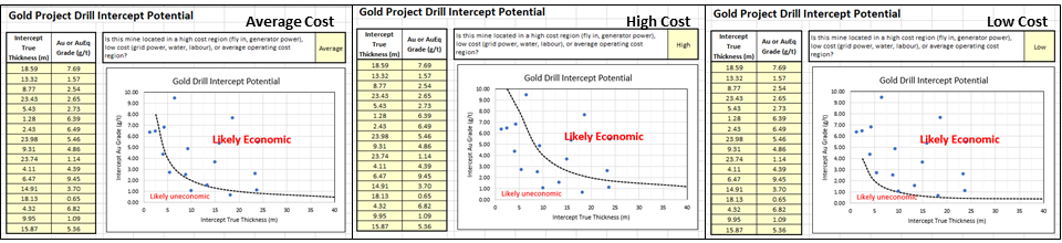
The following charts describe how it works, using randomly generated dummy assay data in this example.
In the Average cost scenario (left chart) the points are equally scattered both above and below the Likely Economic line. As one moves to a high-cost situation (middle chart) the curve moves upwards and more drill intervals now fall below the economic line.
This would give me an unfavorable impression of the project. The third graph is the Low-Cost scenario and one can see that more assays are now above the line. Hence the same project located in a different region would yield a different economic impression.
The economic boundaries (dashed lines) presented in the plots are based on my personal experience and biases. Other people may have different criteria to define what they would view as economic and uneconomic intervals.
Conclusion
There is not much that a layperson person can do with the multitude of exploration data provided in corporate news releases. However, by aggregating the data one can get a sense of where a gold project positions itself economically. The more data points available, the more that one can gather from the plot.
One should prepare separate plots for shallow and deep mineralization or for different zones and deposits on a property rather than aggregate everything together.
It may be possible to undertake a similar analysis with different commodities if one can summarize the assays into a single equivalent value or NSR dollar value. Unfortunately, exploration news releases don’t often include the poly-metallic interval equivalent grade or NSR value. Calculating these manually would add an extra step in the process, however it can be done.
If you want to try out the concept, I have posted the online spreadsheet to my website at the link Drill Intercept Potential where you can input Au exploration data of interest. Unfortunately, you cannot save your input data so it’s a one time event. Anyone can do this – its not rocket science.
Let me know your thoughts, suggestions, or other ways to play with news release data.
If your project contains metals other than gold, then the rock (or ore) value will be based on the revenue from a combination of metals. How to approach this in discussed in another blog post titled “Ore Value Calculator – What’s My Ore Worth?“
Great Bear Resources Example
Interesting the Great Bear Resources website allows one to download a data file with all their exploration intervals. I have not seen another company provide this level of transparency. I download their data file of over 1300 intervals and sub-divided them into major intervals and sub-intervals (more ore less). The two plots below show the outcome.
The graph on the left is the sub-intervals showing that many points are above the “economic” line. There are numerous data points along the top axis, indicating many sub-intervals at >10 g/t at widths ranging from 1 to 15 metres. The graph on the right shows the major intervals. While there are still many along the top axis, there are now more along the 40m width but at grades ranging from 1 g.t to 6 g/t.
One would surmise from these plots that overall there are many intervals above the line in the economic zone, showing the potential of the project. It also shows that GBR have encountered many intervals likely sub-economic, but that’s the exploration game.

Great Bear Resources data
Examining polymetallic drill results in a similar manner isn’t as simple as this. The mutiple metals of interest make the calaculations a bit more complex. Another blog post discusses the approach I use for polymetallic, at this this link “Polymetallic Drill Results – Interesting or Not?“
Note: You can sign up for the KJK mailing list to get notified when new blogs are posted. Follow me on Twitter at @KJKLtd for updates and insights.

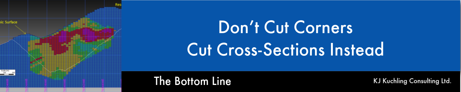
 This article is about the benefit of preparing (cutting) more geological cross-sections and the value they bring.
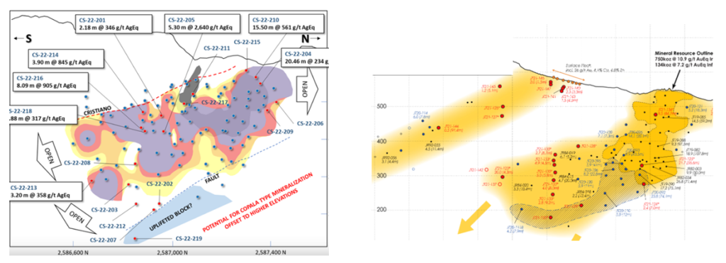 Long sections are aligned along the long axis of the deposit. They can be vertically oriented, although sometimes they may be tilted to follow the dip angle of an ore zone.
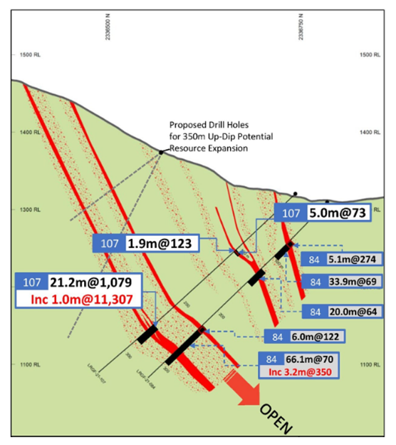
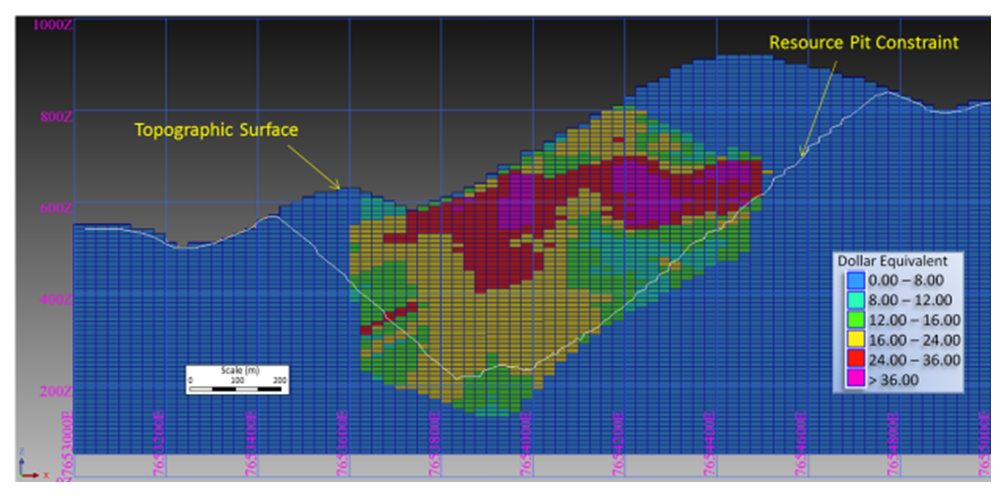 Cross-sections are generally the most popular geological sections seen in presentations. These are vertical slices aligned perpendicular to the strike of the orebody. They can show the ore zone interpretation, drill holes traces, assays, rock types, and/or color-coded resource block grades.
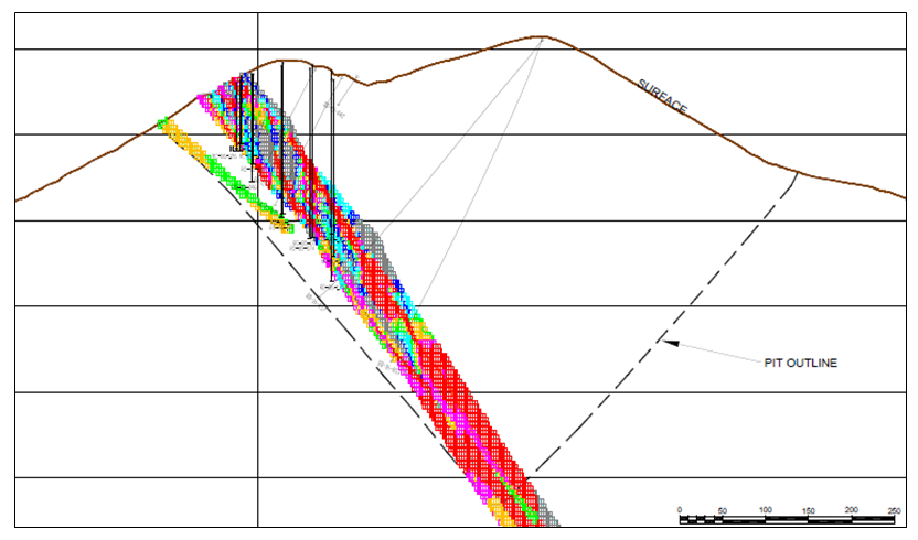 When looking at cross-sections, it is always important to look at multiple cross-sections across the orebody. Too often in reports one may be presented with the widest and juiciest ore zone, as if that was typical for the entire orebody. It likely is not typical.
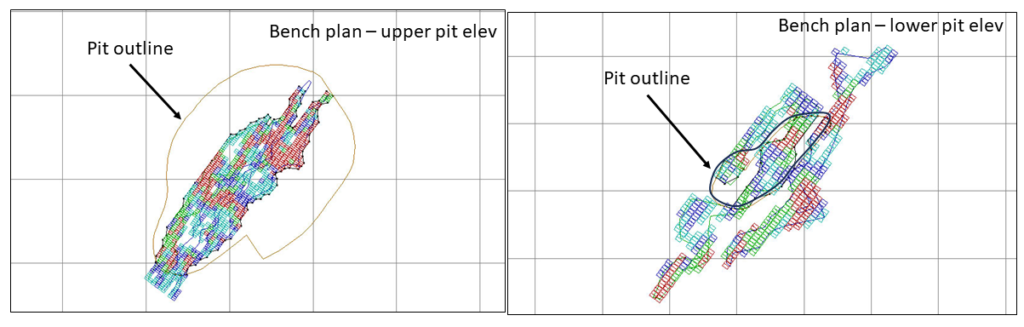 Bench plans (or level plans) are horizontal slices across the ore body at various elevations. In these sections one is looking down on the orebody from above.
 3D PDF files can be created by some of the geological software packages. They can export specific data of interest; for example topography, ore zone wireframes, underground workings, and block model information. These 3D files allows anyone to rotate an image, zoom in as needed and turn layers off and on.
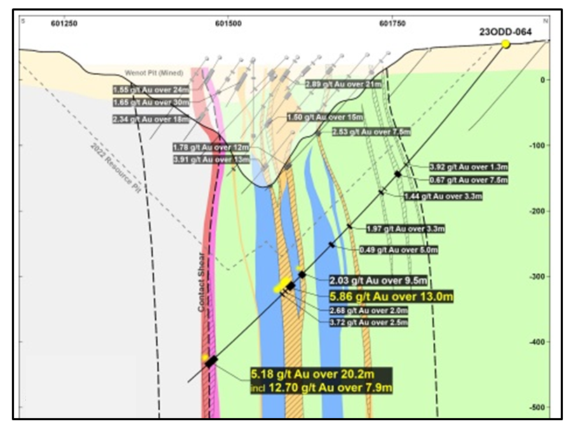 The different types of geological sections all provide useful information. Don’t focus only on cross-sections, and don’t focus only on one typical section. Create more sections at different orientations to help everyone understand better.


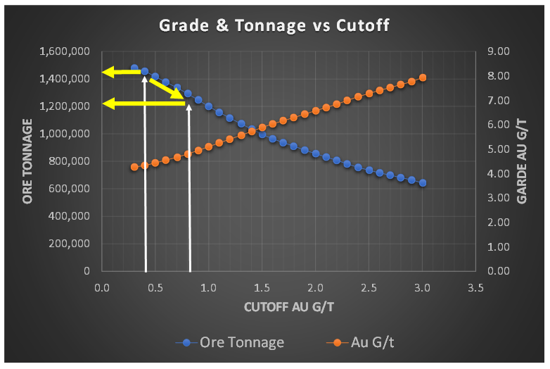 When I am undertaking a due diligence review or working on a study, very early on I like to have a look at the grade-tonnage information. This could be for the entire deposit resource, within a resource constraining shell, or in the pit design.
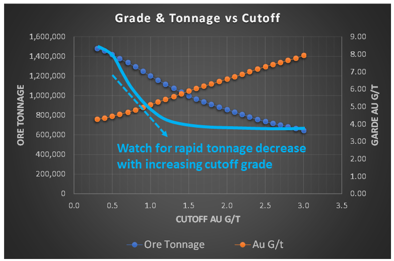 However, if the tonnage curve profile resembled the light blue line in this image, with a concave shape, the ore tonnage is decreasing rapidly with increasing cutoff grade. This is generally not a favorable situation.
 One complaint I have about reporting mineral resources inside a resource constraining shell is the lack of strip ratio information. This applies whether disclosing a single mineral resource estimate or variable grade-tonnage data.
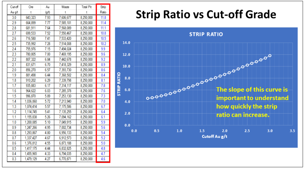 Regarding mineral resources, one should be required to disclose the waste tonnage and strip ratio when reporting resources inside a constraining shell. The constraining shell and cutoff grade are both based on defined economic factors such as unit mining costs, processing cost, process recoveries, and metal prices. With respect to the mining cost component, the strip ratio is a key aspect of the total mining cost, yet it normally isn’t disclosed.
 In 43-101 technical reports, the financial Chapter 22 normally presents the project sensitivities expressed in a spider diagram or a table format.
 When disclosing polymetallic drill results, many companies will convert the multiple metal grades into a single equivalent grade. I am not a big proponent of that approach.
 The three aspects that interest me the most when looking at early-stage drill results are:
 The “NSR factor” would now be 85% x 85% or 75%. Therefore, if the breakeven cost is $14/t, then one should target to mine rock with an insitu value greater than $20/tonne (i.e. $14 / 0.75). This would be the approximate ore vs waste cutoff. It is still only ballpark estimate at this early stage, but good enough for this type of review.


 This might be better than each company applying their own unique equivalent grade calculation to their exploration results.
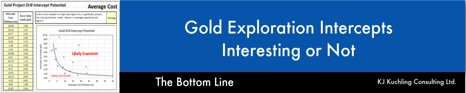

 The algorithm then examines the cell data to teach itself which attributes correlate to known mineralization and which attributes correlate with barren areas. It essentially determines a geological “signature” for each mineralization type. There could be millions of data points and combinations of attributes. Correlation patterns may be invisible to the naked eye, but not to the computer algorithm.
 I was told that many in the geological community tend to discount the AI approach. Either they don’t think it will work or they are fearing for their jobs. Personally I don’t understand these fears nor can I really see how geologists can ever be eliminated. Someone still has to collect and prepare the data as well as ultimately make the final decision on the proposed targets. I don’t see the downside in using AI as another tool in the geologist’s toolbox.

 I like the concept that Globex are promoting. I like the idea of having a one-stop shop that acquires and options out exploration properties to mining companies looking for new projects.

 Do the opposite
 Different companies have different corporate objectives and each mining project will be unique with regards to the impacts of cutoff grade changes on the orebody.
 Tailings dam stability is so important that in some jurisdictions regulators may be requiring that mining companies have third party independent review boards or third party audits done on their tailings dams. The feeling is that, although a reputable consultant may be doing the dam design, there is still a need for some outside oversight.
 Nowadays most small companies do not develop their own in-house resource estimates. The task is generally awarded to an independent QP.
 One downside to a third party review is the added cost to the owner.