

 Recently I have been reviewing a few mining projects from an investor’s perspective. This led me to wonder whether junior mining companies should share more than just their drill hole highlights. What about the raw assays? A mining company announces highlighted drill intervals, but what exactly do those numbers represent?
The highlighted drill interval is based on a series of individual assay samples. The selection of the interval “From” and “To” and “Including” is made by the company using their own criteria. They may include low-grade sections (i.e. smoothing), apply variable cutoffs, sometimes use metal equivalent grades or NSR value to defines the ore/waste cutoff.
The interval definition process is largely invisible to investors, yet for early-stage projects, drill hole intervals are the primary driver of investor communications and their own project valuation.
The underlying basis for drill intervals are raw assay data. These assays can be complex, messy, technical, and may require expertise to interpret properly. However examining the individual assay data can tell more of the story than looking at intervals alone. For example, assays will demonstrate the grade continuity, any nugget effects, or whether thin high-grade spikes are boosting average grades.
This raises the question of whether companies should routinely publish, in CSV format, for download BOTH interval data and raw assay data.
This blog post discusses the pros and cons of releasing assay data electronically.
Why Might an Investor Want the CSV Data
 There is a sense that many mining investors are becoming more sophisticated, and they want to fully understand the exploration process.
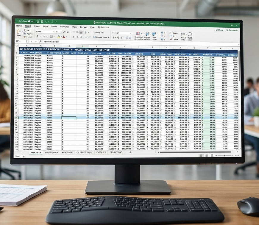
Some investors have geological software with which to examine the exploration data in 3D. Other investors may simply rely on Excel to run their own statistics. Investors may wish to verify what a company is doing, as well as examine their own concept for a project.
Investors might be questioning whether:
-
Companies change the nature of a deposit by smoothing narrow high grade intervals over wider intervals to give the impression of a large tonnage bulk deposit;
-
Companies are using by-product metals in their metal-equivalent, which investors have less confidence in. Perhaps they would prefer to examine the deposit based solely on their primary metals of interest. Perhaps investors prefer to understand the NSR Rock Value ($/t) instead of relying metal-equivalent grades.
-
Companies have not provided sufficient geological cross-sections or 3D images, and investors wish to create their own.
To examine any of these issues, one must have the exploration data in electronic format. For large players, signing an NDA (Non-Disclosure Agreement) and entering the corporate data room provides preferential access to this information. Small players may not be able to do this and some may consider this unfair and selective disclosure.
Highlighted Interval Data in CSV Format
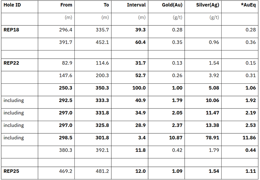
Companies will disclose all highlighted drill INTERVALS in news releases, usually in table format (see example image). If someone wishes to analyze all the interval data on a project, it can be a tedious process to gather all the new releases PDF’s. The tabular data can then be scraped using Ai or one can use Excel “Get Data” functionality on a table by table basis.
This work can be cumbersome and sometimes data does not transform cleanly, often with missing rows, columns, or misaligned data.
Why make investors jump though those hoops to summarize data that’s already been disclosed? Hence, I would suggest companies maintain downloadable historical drill interval data in CSV format on their websites, in a format as presented in the news releases.
Raw assay data, however, is a different matter than interval data since assays have not been made public in the news releases. This is discussed in the next section.
Raw Assay Data in CSV Format
Deciding whether to release raw drill hole assay data is a balance between transparency and strategic risk. The only companies that are doing this (that I am aware of) is Power Metallic and (previously) Great Bear Resources. There may be more that i am not privy to.
There are both pros and cons to making the raw assay data available. Note that raw assay data files typically will also include drill hole collar coordinates and downhole survey information, the whole package.
The Pro’s and Benefits of Raw Data Disclosure
1. Market Credibility: A company being “radically transparent” can set them apart by signaling to the market confidence in their data and they have nothing to hide. This can build trust with those who want to verify the discovery. This can differentiate one from peers in a crowded junior market where transparency may be lacking.
2. Free Technical Analysis: Raw data appeals to technically sophisticated investors, geologists, and analysts who want to do their own review. The independent “super-investors” who run their own models may reach the same conclusions as the company, proving external validation for the project. They may essentially help IR with free marketing and 3rd party promotion. Of course, the opposite can also happen if the project is not as robust as being promoted by the company.
3. Speed: Raw data access may speed up due diligence for potential acquirers or JV partners who can initiate confidential internal reviews prior to deciding whether to enter a formal NDA and due diligence process.
The Con’s and Risks of Raw Data Disclosure
 1. Misinterpretation & “Amateur” Experts: One risk is that someone with a very basic understanding of mining software and limited understanding of the local geology, runs flawed interpretations and publicizes their incorrect conclusions. A company may find that correcting false narratives publicly can be harder than preventing them.
Conversely stock pumpers can cherry-pick individual high-grade intervals out of context and also create misleading narratives (albeit positive) outside of the company control. They may have their own motives to pump the stock.
2. Competitive Intelligence: If in a competitive exploration district, neighbors can use raw assay values and lithology codes to predict where the mineralization is trending. This could help them acquire adjacent mineral claims before one can fully consolidate the regional land package. Regardless, competitors may still be able to do some of this using the drill hole interval data from news releases, so this may not be a big risk.
3. Liability and Compliance: NI 43-101 reporting requires technical data to be verified by a Qualified Person (QP). If one provides a raw assay file that isn’t properly vetted or contains errors, will there be regulatory or legal issues? Normally a corporate QP signs off on news releases, not necessarily an independent QP.
There have also been cases where assay data has been purposely manipulated from lab certificates to the drill hole database, and investors would then be working with this falsified data. Corporate liability could be a big risk in the eyes of some.
The Assay Disclosure Middle Ground
 Once the assay data is public, it may be more difficult for a company to manage the story. A press release lets them frame results in the context of their business plan; a raw data file does not.
Instead of providing a full assay database download, some companies might follow the approach below. It may not satisfy everyone, but could be better than just ignoring requests for more detailed information.
-
Interactive Map: Use a web-based GIS tool that allows users to click holes and see downhole results graphically without downloading the full database.
-
Cross-Sections: Provide multiple high-quality cross-sections that show the geological interpretation alongside the raw assay grades or use a grade bar chart along the drill hole trace. This provides information on the grade continuity and uniformity without releasing the actual grades.
-
Post-resource estimate disclosure: Once the database has been formally audited by an independent QP and incorporated into a 43-101 technical report for a resource estimate, releasing the assay data may be lower risk.
These actions may give a sense of greater transparency while keeping the raw data within a controlled environment. It will help prevent amateurs from erroneous modeling the geology yet still “somewhat” satisfying the sophisticated mining investor.
Conclusion
 For investors trying to assess a junior explorer, or geologists conducting a technical review, or a regulator trying to ensure fair and accurate disclosure, access to raw assay data can play a part in promoting good judgment and accurate disclosure from companies.
However some suggest that raw data without context is subject to misinterpretation.
Personally, I would prefer to see the release of both drill intervals and raw assay tables in CSV format.
In this modern area of Ai and investor sophistication, greater data transparency may be a positive and help build more trust in the industry. However, I understand the reasons not to do this and understand if companies choose to not go this route.
Currently the mining industry norm is that raw assays stay in private data rooms and not on corporate websites. Credibility tries to be achieved via clear, technically detailed news releases and Technical Reports.
In case you missed it, the last blog post was “What Does Ai Think of Toll Milling“.
You can sign up for the KJK mailing list to get notified when new blogs are posted. Follow me on Twitter at @KJKLtd for updates and other mining posts. The entire blog post library can be found at https://kuchling.com/library/
APPENDIX: EXCEL TASKS with and ASSAY DATABASE
I asked an Ai colleague Claude to list all the things one could do in Excel with publicly released drill hole information. Here is what it said (unedited). Its never lacking in advice and Claude will even help you create the Excel worksheet logic if needed.
Grade Analysis
-
Descriptive statistics – mean, median, mode, min/max, standard deviation of assay values (Au, Ag, Cu, etc.)
Grade frequency distributions — histogram charts to understand grade population shape.
-
High-grade outlier identification — flagging values above a threshold (e.g., >3x median) that may need capping consideration.
-
Grade capping/cutting analysis — testing different cap values and their effect on average grade.
-
Coefficient of Variation (CV) — assessing grade variability and nugget effect risk.
Composite & Interval Analysis
-
Downhole compositing — averaging assay intervals into fixed-length composites (e.g., 2m or 5m) using weighted averages.
-
True width estimation — applying trigonometric corrections for hole dip/azimuth vs. vein orientation.
Grade x thickness (GT) calculations — multiplying average grade by intercept width for comparative ranking of intersections.
-
Cut-off grade sensitivity — running intercept calculations at multiple cut-off grades to see how reported widths and grades change.
Hole Correlation & Comparison
-
Hole-by-hole grade comparison — ranking holes by peak grade, average grade, or GT value.
-
Section-by-section comparison— grouping holes by fence/section for along-strike trend analysis.
-
Depth vs. grade plots — scatter plots to look for grade zonation with depth.
-
Multi-element ratio analysis— e.g., Au:Ag ratios, Cu:Mo ratios to identify metallogenic zonation or alteration trends.
Spatial & Trend Analysis
-
Collar location plotting — basic X/Y scatter plots of collar coordinates to visualize drill pattern coverage.
-
Downhole survey data — using dip/azimuth measurements to approximate downhole trace (basic desurveying).
-
Strike and dip trend identification — plotting grade against easting or northing to identify directional trends.
-
Variogram-lite analysis — plotting grade vs. distance between holes to get a rough sense of spatial continuity (proper variography needs dedicated software).
Multi-Element & Geochemical Analysis
-
Correlation matrices — identifying which elements are positively or negatively correlated (e.g., Au vs. As in a Carlin-type system).
-
Scatter plots — visualizing element-pair relationships to identify pathfinder associations.
-
Log-transformation — applying LOG10 to skewed assay data before statistical analysis, which is standard practice.
-
Anomaly thresholding— mean + 2 standard deviations as a simple anomaly threshold for pathfinder elements.
Resource Estimation (Basic)
-
Polygonal area calculations — basic area-of-influence resource estimation using drill spacing geometry.
-
Grade tonnage curves — plotting tonnes vs. grade at varying cut-offs using simplified volume assumptions.
-
Bulk density sensitivity** — testing how different SG assumptions affect tonnage estimates.
Reporting & QA/QC
-
Duplicate analysis — comparing field duplicate, coarse reject duplicate, and pulp duplicate pairs using scatter plots and % relative difference calculations.
-
Standard performance tracking — plotting certified reference material (CRM) results against expected values and control limits (±2SD, ±3SD).
-
Blank monitoring — flagging blank samples that exceed contamination thresholds.
-
Laboratory turnaround tracking — monitoring submission dates vs. return dates.


 I recently noticed a few new mining studies that relied on toll milling as their base case operation. This made me wonder if this is a trend and if there are more examples of where this is happening.
 USER PROMPT: What are the risks of toll milling plan.
 RESPONSE: The Qualified Person (QP) signing off on a technical study that uses toll milling as the base case carries significant professional and regulatory responsibility, particularly under NI 43-101 in Canada or JORC in Australia.
 The results given by Claude are quite thorough and insightful. It’s hard to argue with its observations and conclusions. This research took all of 30 seconds, so I can see it is no longer difficult to become a blog writer. Writing isn’t the challenge; finding interesting topics is.
 The lesson is that QP’s signing off on technical information for clients should be proficient in the nature of their work and need to know the reporting rules very well. Some of these incidents involve error and poor judgment, not outright fraud.
 43-101 regulations state that “An issuer must not file a technical report that contains a disclaimer by any qualified person responsible for preparing or supervising the preparation of all or part of the report that
 This ends Part 2 of this blog post. It hopefully highlights the importance of QP’s being knowledgably on the disclosure rules and the technical aspects of what they are hired to do.
 The focus of this blog is on the types of activities that raised the red flags in the past. I am less interested in naming the people responsible, although the associated web links do provide more detail on the events.
 This ends Part 1 of this blog post. Part 2 will continue with a few more examples, specifically involving Qualified Persons, and can be found at this link
 So, you just completed your initial PEA cashflow model and the resulting NPV and IRR are a little disappointing. They are not what everyone was expecting. They don’t meet the ideal targets of an IRR greater than 30% and an NPV that is more than 2x the initial capital cost. The project could now be on life support in the eyes of some.
 The discounting of cashflows in a cashflow model means that up-front revenues and costs have a bigger impact on the final economics than those far off in the future. This effect is amplified at higher discount rates.
 ake to the cashflow model. Sometimes several of the small ones, when compounded together, will result in a significant impact. Here are some of the other cashflow model adjustments that I have seen.
 Don’t let a disappointing NPV get you down. There may be a few ways to boost the NPV by applying some common practices. However, if after applying all of these adjustments, the NPV still isn’t great, something bigger may be required. That could be an entire project scope re-think.
 Two dilution approaches are common. One can either construct a diluted block model; or one can apply dilution afterwards in the production schedule. I have used both approaches at different times.
 Sometimes lower grade stockpiles are built up by the mine each year but only processed at the end of the mine life. Periodically the ore mining rate may exceed the processing rate and other times it may be less. This is where the stockpile provides its service, smoothing the ore delivery to the plant.
 Once the schedules are finalized, they are normally reviewed by the client for approval. The strip ratio and ore grade profile by date are of interest. One may then be asked to look to at different stockpiling approaches to see if an NPV (i.e. head grade) improvement is possible.
 The last task for the mine engineer in Chapter 16 is estimating the open pit equipment fleet and manpower needs. The capital and operating costs for the mining operation will also be calculated as part of this work, but the costs are only presented in Chapter 21.
 The support equipment needs (dozers, graders, pickups, mechanics trucks, etc.) are typically fixed. For example, 2 graders per year regardless if the annual tonnages mined fluctuate.
 These two blog posts hopefully give an overview of some of the things that mining engineers do as part of their jobs. Hopefully the posts also shed light on the amount of work that goes into Chapter 16 of a 43-101 report. While that chapter may not seem that long compared to some of the others, a lot of the effort is behind the scenes.
 So I thought what better way to explain the mining engineer role than by describing the anatomy of a typical Chapter 16 (MINING) in a 43-101 Technical Report. That chapter is a good example of the range of tasks typically undertaken by mining engineers.
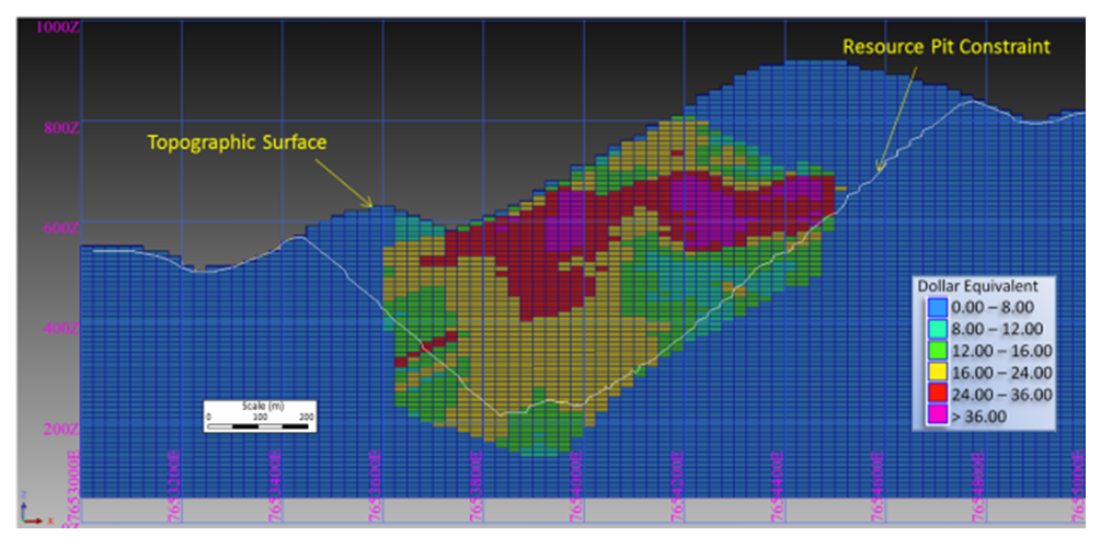 There is always a mineral resource estimate available before doing a PEA. The way the resource is reported will indicate what type of mine this likely is. The geologists have already done some of the mining engineer’s work.
 Before starting pit optimization, we require economic inputs from several people. The base case metal prices must be selected (normally with input from the client). The mining operating cost per tonne must be estimated (by the mining engineer). The processing engineers will provide the processing cost and recovery for each ore type.
 Once the optimization is run, a series of nested pit shells are created, each with its own tonnes and grade. These shells are compared for incremental strip ratio, incremental head grade, total tonnes, and contained metal.
 The mining engineer is now ready to undertake the pit design. The pit design step introduces a benched slope profile, smooths out the pit shape, and adds haulroads. Hence a couple of key input parameters are required at this time. The mining engineer will need to know the geotechnical pit slope criteria and the truck size & haul road widths. Let’s look at both of these.
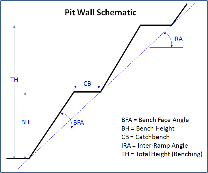
 Ramps: Next the mining engineer needs to select the truck size, even though the production schedule has not yet been created.
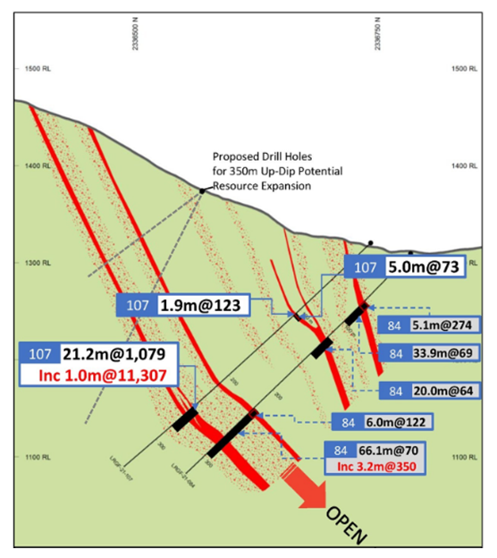 This article is about the benefit of preparing (cutting) more geological cross-sections and the value they bring.
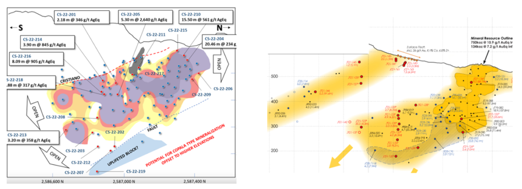 Long sections are aligned along the long axis of the deposit. They can be vertically oriented, although sometimes they may be tilted to follow the dip angle of an ore zone.
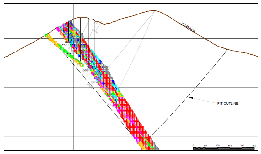 When looking at cross-sections, it is always important to look at multiple cross-sections across the orebody. Too often in reports one may be presented with the widest and juiciest ore zone, as if that was typical for the entire orebody. It likely is not typical.
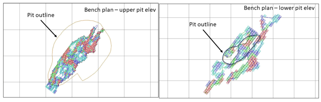 Bench plans (or level plans) are horizontal slices across the ore body at various elevations. In these sections one is looking down on the orebody from above.
 3D PDF files can be created by some of the geological software packages. They can export specific data of interest; for example topography, ore zone wireframes, underground workings, and block model information. These 3D files allows anyone to rotate an image, zoom in as needed and turn layers off and on.
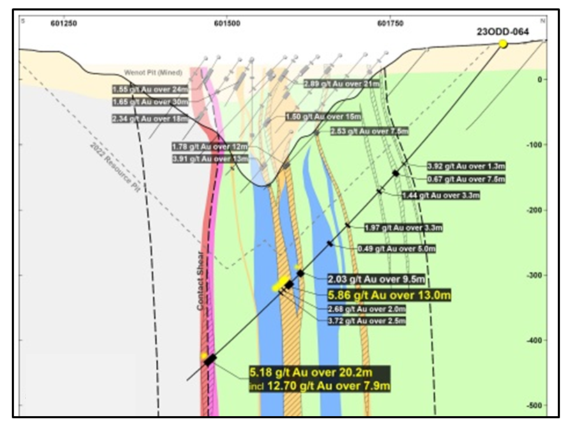 The different types of geological sections all provide useful information. Don’t focus only on cross-sections, and don’t focus only on one typical section. Create more sections at different orientations to help everyone understand better.


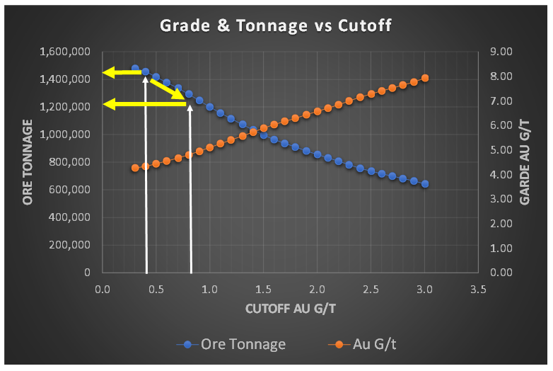 When I am undertaking a due diligence review or working on a study, very early on I like to have a look at the grade-tonnage information. This could be for the entire deposit resource, within a resource constraining shell, or in the pit design.
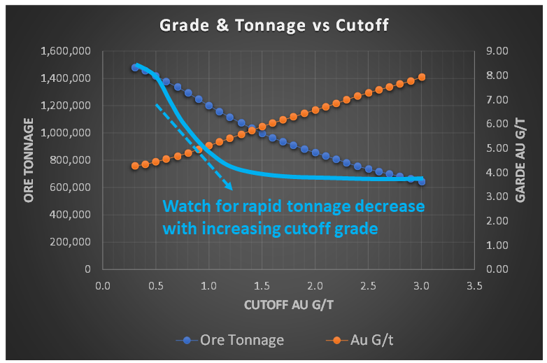 However, if the tonnage curve profile resembled the light blue line in this image, with a concave shape, the ore tonnage is decreasing rapidly with increasing cutoff grade. This is generally not a favorable situation.
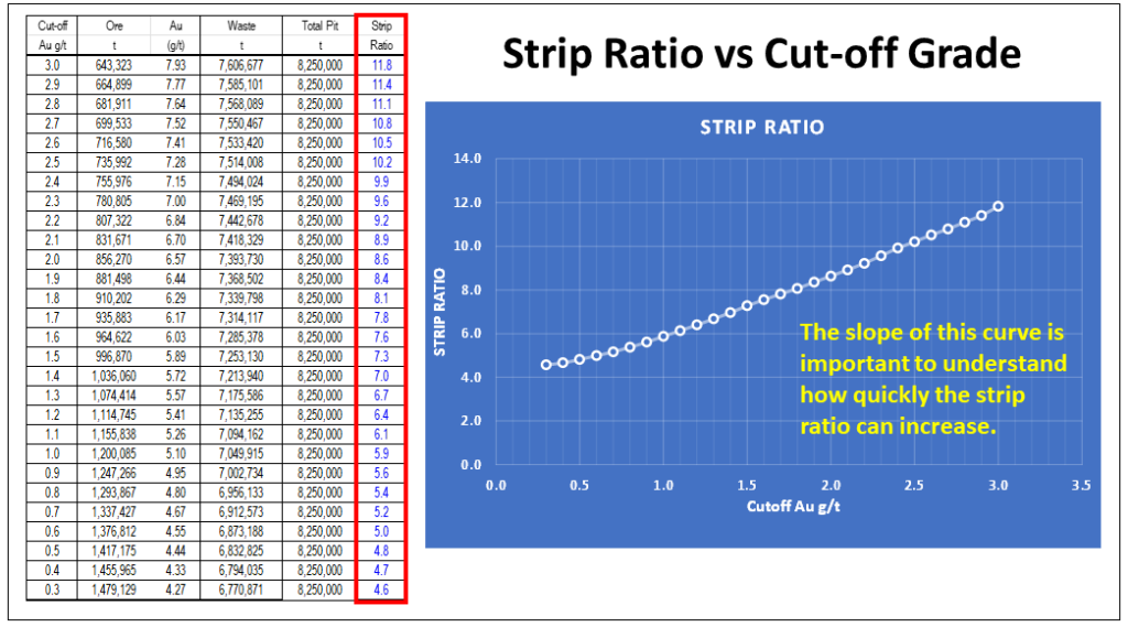 Regarding mineral resources, one should be required to disclose the waste tonnage and strip ratio when reporting resources inside a constraining shell. The constraining shell and cutoff grade are both based on defined economic factors such as unit mining costs, processing cost, process recoveries, and metal prices. With respect to the mining cost component, the strip ratio is a key aspect of the total mining cost, yet it normally isn’t disclosed.
 In 43-101 technical reports, the financial Chapter 22 normally presents the project sensitivities expressed in a spider diagram or a table format.
 When disclosing polymetallic drill results, many companies will convert the multiple metal grades into a single equivalent grade. I am not a big proponent of that approach.
 The three aspects that interest me the most when looking at early-stage drill results are:
 The “NSR factor” would now be 85% x 85% or 75%. Therefore, if the breakeven cost is $14/t, then one should target to mine rock with an insitu value greater than $20/tonne (i.e. $14 / 0.75). This would be the approximate ore vs waste cutoff. It is still only ballpark estimate at this early stage, but good enough for this type of review.


 This might be better than each company applying their own unique equivalent grade calculation to their exploration results.