
 This article is about the benefit of preparing (cutting) more geological cross-sections and the value they bring.
Geological sections are one of the easiest ways to explain the character of an orebody. They have an inherent simplicity yet provide more information than any other mining related graphic.
Some sections can be simple cartoon-like images while others can be technically complicated, presenting detailed geological data.
Cartoon-stylized sections are typically used to describe the general nature of the orebody. The detailed sections can present technical data such as drill hole traces, color coded assays intervals, ore block grades, ore zone interpretations, mineral classifications, etc.
Sections provide a level of clarity to everyone, including to those new to the mining industry as well as those with decades of experience.
This article briefly describes what story I (as an engineer) am looking for in sections. Geologists may have a different view on what they conclude when reviewing geological sections.
I will describe the three types of geological sections that one can cut and what each may be describing. The three types are: (1) longitudinal (long) sections; (2) cross-sections; (3) bench (level) plans. Each plays a different role in helping to understand the orebody and mining environment.
There is also another way to share simple geological images via3D PDF files. I will provide an example later.
Longitudinal (Long) Sections
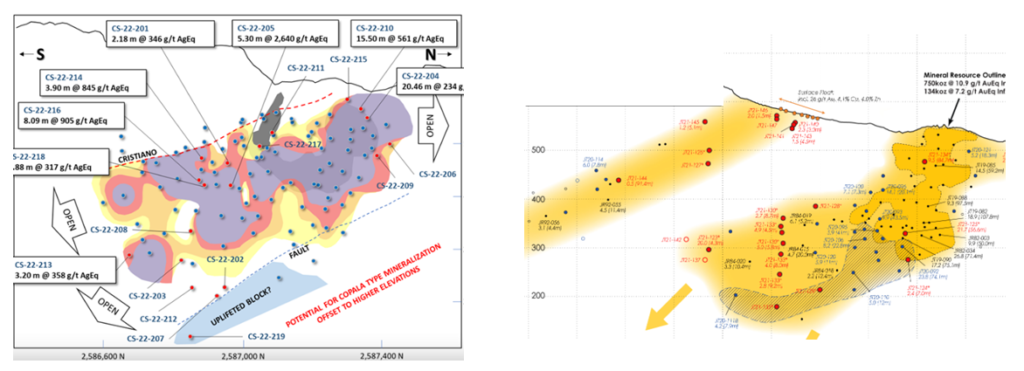 Long sections are aligned along the long axis of the deposit. They can be vertically oriented, although sometimes they may be tilted to follow the dip angle of an ore zone.
Long sections are typically shown for narrow structure style deposits (e.g. gold veins) and are typically less relevant for bulk deposits (e.g. porphyry).
The information garnered from long sections includes:
-
The lateral extent of the mineralized structure, which can be in hundred of metres or even kilometers. This provides a sense for how large the entire system is. Sometimes these sections may show geophysics, drilling to defend the basis for the regional interpretation.
-
Long sections will often highlight the drill hole pierce points to illustrate how well the mineralized zone is drilled off. Is the ore zone defined with a good drill density or are there only widely spaced holes? As well, long sections can show how deep ore zone has been defined by drilling. On some projects, a few widely spaced deep holes, although insufficient for resource estimation purposes, may confirm that the ore zone extends to great depth. This bodes well for potential development in that a long life deposit may exist.
-
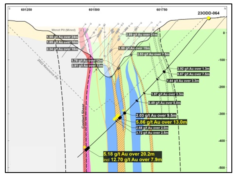
Sometimes the long section drill intercept pierce points can be contoured on grade, thickness, or grade-thickness. This information provides a sense for the uniformity (or variability) of the ore zone. It also shows the elevations of the higher grade zones, if the deposit is more likely an open pit mine, an underground mine, or a combination of both.
Cross-Sections
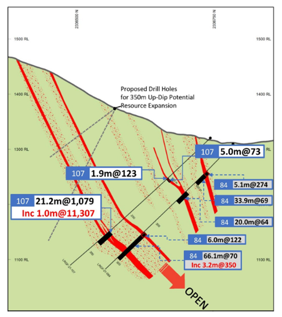
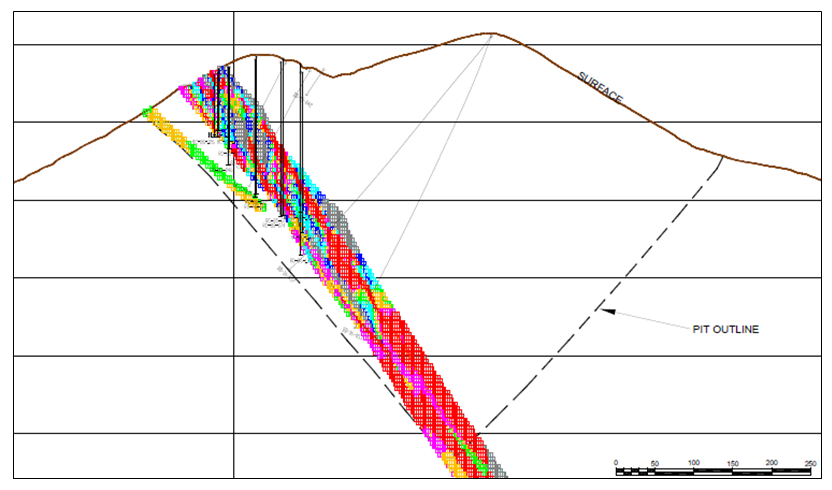
 Cross-sections are generally the most popular geological sections seen in presentations. These are vertical slices aligned perpendicular to the strike of the orebody. They can show the ore zone interpretation, drill holes traces, assays, rock types, and/or color-coded resource block grades.
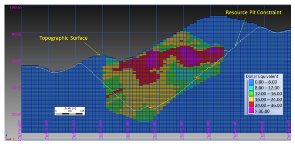
As an engineer, my greatest interest is in seeing the resource blocks, color coded by grade. Sometimes open pit shells may be included on the section to define the potential mining volume. The engineering information garnered from block model cross-sections includes:
-
Where are the higher-grade areas located; at depth or near surface?
-
If a pit shell profile is included, what will the relative strip ratio look like? Are the ore zones relatively narrow compared to the size of the pit?
-
How will the topography impact on the pit shape? In mountainous terrain, will a push-back on pit wall result in the need to climb up a hillside and create a very high pit slope? This can result in high stripping ratios or difficult mining conditions.
-
Does the ore zone extend deeper and if one wants to push the pit a bit deeper, is there a high incremental strip ratio to do this? Does one need to strip a lot of waste to gain a bit more ore?
-
Are the widths of the mineable ore zones narrow or wide, or are there multiple ore zones separated by internal waste zones? This may indicate if lower-cost bulk mining is possible, or if higher cost selective mining is required to minimize waste dilution.
-
How difficult will it be to maintain grade control? For example, narrow veins being mined using a 10 metre bench height and 7 metre blast pattern will have difficulty in defining the ore /waste contacts.
-
Cross-sections that show the ore blocks color coded by classification (Measured, Indicated, Inferred), illustrate where the less reliable (Inferred) resources are located and how much relative tonnage may be in the more certain Measured and Indicated categories.
 When looking at cross-sections, it is always important to look at multiple cross-sections across the orebody. Too often in reports one may be presented with the widest and juiciest ore zone, as if that was typical for the entire orebody. It likely is not typical.
Stepping away from that one section to look at others is important. Possibly the character of the ore zones changes and hence its important to cut multiple sections along the orebody.
Bench (Level) Plans
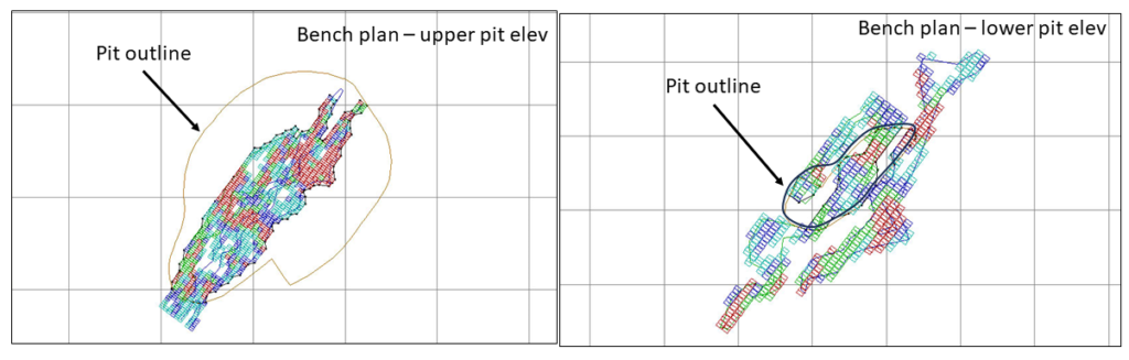 Bench plans (or level plans) are horizontal slices across the ore body at various elevations. In these sections one is looking down on the orebody from above.
Level plans are typically less common to see in presentations, although they are very useful. The level plans may show geological detail, rock types, ore zone interpretations, ore block grades, and underground workings.
The bench plan represents what the open pit mining crews would see as they are working along a bench in the pit. The information garnered from bench plans that include the block model grades includes:
-
Where are the higher-grade areas found on a level? Are these higher grade areas continuous or do they consist of higher grade pockets scattered amongst lower grade blocks?
-
Do the ore zones swell or pinch out on a bench? A vertical cross-section may give a false sense the ore zones are uniform. The bench plan gives an indication on how complicated mining, grade control, and dilution control might be for operators.
-
Do the ore zones on a bench level extend out beyond the pit walls and is there potential to expand the pit to capture that ore?
-
On a given bench what will the strip ratio be? Are the ore zones small compared to the total area of the bench?
As recommended with cross-sections, when looking at bench plans, one should try to look at multiple elevations. The mineability of the ore zones may change as one moves vertically upwards or downwards through a deposit.
Never mind cross-sections – give me 3D
While geological sections are great, another way to present the orebody is with 3D PDF files to allow users to view the deposit in three-dimensions. Web platforms like VRIFY are great, but I have been told they sometimes can be slow to use.
 3D PDF files can be created by some of the geological software packages. They can export specific data of interest; for example topography, ore zone wireframes, underground workings, and block model information. These 3D files allows anyone to rotate an image, zoom in as needed and turn layers off and on.
You can also create your own simplistic cross-sections through the pdf menus (see image).
A simple example of such a 3D PDF file can be downloaded at this link (3D DPF File Example). It only includes two pit designs and some ore blocks to keep it simple.
The nice thing about these PDF files is that one doesn’t need a standalone viewer program (e.g. Leapfrog viewer) to view them. They are also not huge in size. As far as I know 3D PDF files only work with Adobe Reader, which most everyone already has. It would be good if companies made such 3D PDF files downloadable along with their corporate PowerPoint presentations.
Conclusion
 The different types of geological sections all provide useful information. Don’t focus only on cross-sections, and don’t focus only on one typical section. Create more sections at different orientations to help everyone understand better.
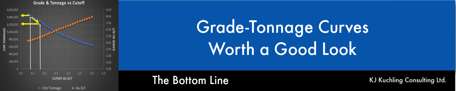


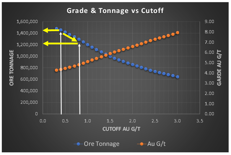 When I am undertaking a due diligence review or working on a study, very early on I like to have a look at the grade-tonnage information. This could be for the entire deposit resource, within a resource constraining shell, or in the pit design.
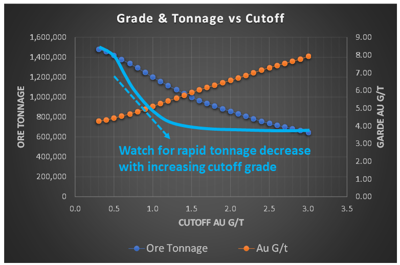 However, if the tonnage curve profile resembled the light blue line in this image, with a concave shape, the ore tonnage is decreasing rapidly with increasing cutoff grade. This is generally not a favorable situation.
 One complaint I have about reporting mineral resources inside a resource constraining shell is the lack of strip ratio information. This applies whether disclosing a single mineral resource estimate or variable grade-tonnage data.
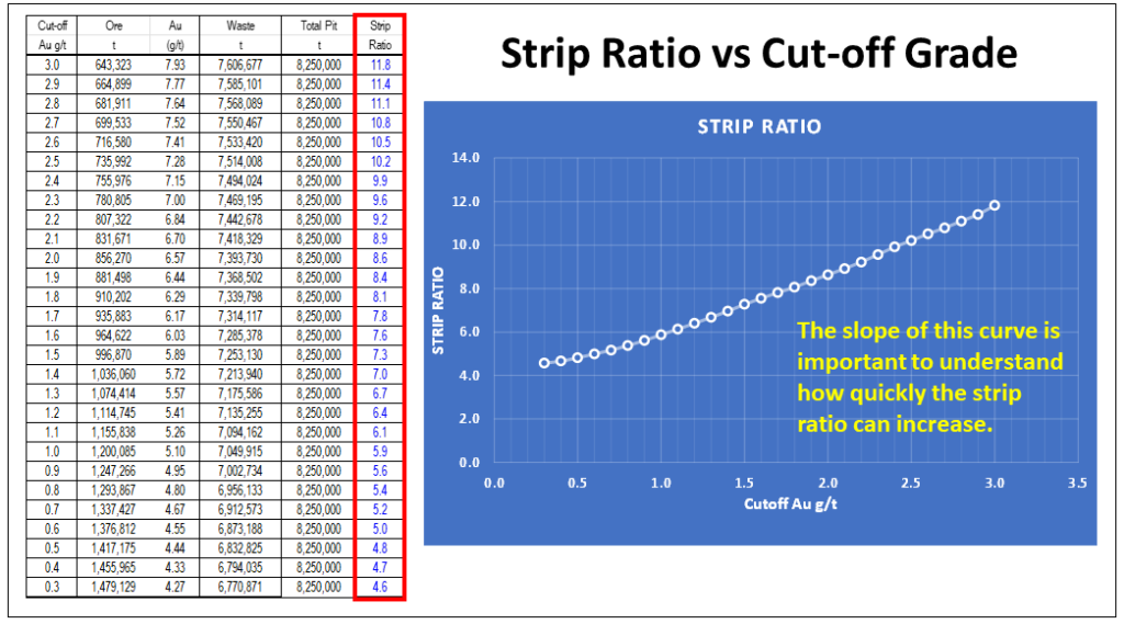 Regarding mineral resources, one should be required to disclose the waste tonnage and strip ratio when reporting resources inside a constraining shell. The constraining shell and cutoff grade are both based on defined economic factors such as unit mining costs, processing cost, process recoveries, and metal prices. With respect to the mining cost component, the strip ratio is a key aspect of the total mining cost, yet it normally isn’t disclosed.
 In 43-101 technical reports, the financial Chapter 22 normally presents the project sensitivities expressed in a spider diagram or a table format.
 When disclosing polymetallic drill results, many companies will convert the multiple metal grades into a single equivalent grade. I am not a big proponent of that approach.
 The three aspects that interest me the most when looking at early-stage drill results are:
 The “NSR factor” would now be 85% x 85% or 75%. Therefore, if the breakeven cost is $14/t, then one should target to mine rock with an insitu value greater than $20/tonne (i.e. $14 / 0.75). This would be the approximate ore vs waste cutoff. It is still only ballpark estimate at this early stage, but good enough for this type of review.


 This might be better than each company applying their own unique equivalent grade calculation to their exploration results.
 The primary question to be answered is whether one can mine safely and economically without creating significant impacts on the environment.
 Lake Turbidity: Dike construction will need to be done through the water column. Works such as dredging or dumping rock fill will create sediment plumes that can extend far beyond the dike. Is the area particularly sensitive to such turbidity disturbances, is there water current flow to carry away sediments?
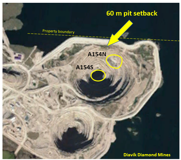 Pit wall setback: Given the size and depth of the open pit, how far must the dike be from the pit crest? Its nice to have 200 metre setback distance, but that may push the dike out into deeper water.
 Once the approximate location of the dike has been identified, the next step is to examine the design of the dike itself. Most of the issues to be considered relate to the geotechnical site conditions.
 Each mine site is different, and that is what makes mining into water bodies a unique challenge. However many mine operators have done this successfully using various approaches to tackle the challenge.
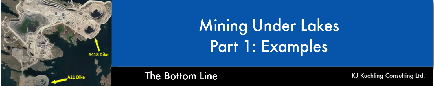


 NPV One is targeting to replace the typical Excel based cashflow model with an online cloud model. It reminds me of personal income tax software, where one simply inputs the income and expense information, and then the software takes over doing all the calculations and outputting the result.
 Pros
Pros Like anything, nothing is perfect and NPV may have a few issues for me.
 The NPV One software is an option for those wishing to standardize or simplify their financial modelling.
 We likely have all heard the statement that increasing pit wall angles will result in significant cost savings to the mining operation.
 The results of applying the increased inter-ramp angle to each of the four pits is shown in the Bar Chart. Note that the waste reduction is not necessarily the same for each pit. It depends on the specific topography around each pit.
 In general one can typically see four positive outcomes from adopting steeper pit walls. They are as follows:
 4. Pit Crest Location: The steeper wall angles result in a shift in the final pit crest location. The Image shows the impact that the 5 degree steepening had on the crest location for one of the pits in this scenario.
 It is relatively easy to justify spending additional time and money on proper geotechnical investigations and geotechnical monitoring given the potential slope steepening benefits.

 I remember in the late fall of that year, the company had a chance to bid on a larger project in Gros Morne National Park, Newfoundland. So our President, Frank Nolan (he was a brother to Fred Nolan, the infamous land-owner at Oak Island, by the way), decided he wanted to see the site and he chartered a Bell 106 helicopter to fly us there from Deer Lake. It was December (they say “December month” in that province) and when we got close to the Park, we ran into a sudden snow squall.
 The QMM field office In Port Dauphin, Madagascar was located near the edge of town, and I typically walked from my lodging to the office each morning when I was there, about the time when school started for the children. Typically I passed dozens and dozens of tiny bamboo huts with corrugated metal roofs, and dirt floors each about 2 meters square.
 It is one thing to briefly visit a remote project as part of a review team. It is another thing to be there as part of a design team trying to solve a problem and engineer a solution. I know of many engineers and geologists that would have similar work life experiences as part of their careers. However John has taken the initiative to write it all down.
 Overburden is a generalized termed used to describe unconsolidated material encountered at a mine. It can consist of gravels, sands, silts, and clays and combinations of each. Usually overburden is not given much focus in many mining studies. Very often, the overburden as a unit, is not adequately characterized.
 These are the clays most people are familiar with, i.e. a sedimentary deposit of very fine particles that have settled in a calm body of water. Normally consolidated clays are generally not a problem, other than having a high moisture content. As such, they can be very sticky in loader buckets, truck boxes, and when feeding crushers.
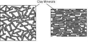 Clays in general consist of very fine plate like particles, as shown in this sketch. In over-consolidated clays, these particles have been flattened and tightly compressed as in the right image. The result is that the clay may be dense, have a good cross bedding shear strength, but very low shear strength along the plates. This characteristic is analogous to the lubricating properties of graphite, which is facilitated by sliding along graphite plates.
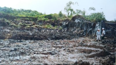 My experience with sensitive clays was at the former BHP bauxite mining operations along the northern coast of Suriname. There were Demerara clay channels up to 20m thick over top of many of their open pits. The bucketwheel excavators used for waste stripping would trigger the quick clay slope failures, sometimes resulting in the crawler tracks being buried and unfortunately also causing some worker fatalities.
 I recall walking up towards a bucketwheel digging face as the machine quietly churned away. About 70 metres from the machine, we would see cracks quietly opening all around us as the ground mass was starting to initiate its flow towards the machine. Most times the bucketwheel could just sit there and dig. Instead of the machine having to advance toward the face, the face would advance towards the machine.
 The formation of the diamond deposits in northern Canada often involved the explosive eruption of kimberlite pipes under bodies of water. The lakebed muds and expelled kimberlite by the eruption would collapse back into the crater, resulting in a mix of mud and kimberlite (yellow zones in the image). This muddy kimberlite could be soft, weak, and difficult to mine with underground methods.
 At many tropical mining operations (west African gold projects for example) the upper bedrock has undergone weathering, resulting in the fresh rock being decomposed into saprolite. This clay-rich material can exceed 50 metres in thickness, can be fairly soft and diggable without blasting. This is an obvious mining cost benefit.
 Compacted clay fill can also be used as a pond liner material for water retention ponds.
 Mining has been a part of my life for as long as I can remember. Being born in Sudbury, many of my family members have been, or are currently involved, in mining through a variety of occupations, including my father who I idolized. However, I never knew my true interest in the industry until my 11th-grade technology class. I had a teacher who was passionate about the mining industry, and he created a project that involved developing a very basic mine design.
 Before my first year of university, I had a summer job tramming at Macassa Mine in Kirkland Lake Ontario, which has been in production since 1933. My mentality was to get the boots on the ground and get the job done, whatever it took (with proper safety precautions of course). Using rail systems, dumping ore cars manually, jackleg drilling, etc. gave me the perspective that mining was archaic, mining was rough, and mining was only about the ounces.
 To change the negative view around mining, I believe the main focal point should be electric equipment and the ability for remote operation/work. With all this newly developed technology at our fingertips, I know that future operations will be safer and more sustainable, which should be better portrayed.
 Even creating a mining simulation video game where you can run through a story of being a manager, excavator/scoop operator, truck driver, etc. would get the thought of mining brought into the coming generations at a younger age. This would increase the talent pool from the more typical operator because more and more youth are getting skilled at remote operation through video games due to their increased screen time.
 People get comfortable and people are afraid to leave home, so selling a career that allows for boundless flexibility in job tasks and constant stimulation while living wherever you desire could allow a shrinkage in the current technical gap.
 So do I think the mining industry is archaic…. not anymore.
 Firstly, I would like to thank this engineer for taking time to write out his well formed thoughts, and for allowing me to share them.