In my view one thing lacking in the mining industry today is a consistent approach to quantifying and presenting the risks associated with mining projects. In a blog written in 2015 titled “Mining Cashflow Sensitivity Analyses – Be Careful” I discussed the limitations of the standard “spider graph” sensitivity analysis often seen in Section 22 of 43-101 reports.
This blog post expands on that discussion by describing a better approach. A six-year time gap between the two articles – no need to rush I guess.
This blog summarizes excerpts from an article written by a colleague that specializes in probabilistic financial analysis. That article is a result of conversations we had about the current methods of addressing risk in mining. The full article can be found at this link, however selected excerpts and graphs have been reprinted here with permission from the author.
The author is Lachlan Hughson, the Founder of 4-D Resources Advisory LLC. He has a 30-year career in the mining/metals and oil gas industry as an investment banker and a corporate executive. His website is here 4-D Resources Advisory LLC.
Excerpts from the article
Mining can be risky
“The natural resources industry, especially the finance function, tends to use a static, or single data estimate, approach to its planning, valuation and M&A models. This often fails to capture the dynamic interrelationships between the strategic, operational and financial variables of the business, especially commodity price volatility, over time.”
“A comprehensive financial model should correctly reflect the dynamic interplay of these fundamental variables over the company life and commodity price cycles. This requires enhancing the quality of key input variables and quantitatively defining how they interrelate and change depending on the strategy, operational focus and capital structure utilized by the company.”
“Given these critical limitations, a static modeling approach fundamentally reduces the decision making power of the results generated leading to unbalanced views as to the actual probabilities associated with expected outcomes. Equally, it creates an over-confident belief as to outcomes and eliminates the potential optionality of different courses of action as real options cannot be fully evaluated.”

Monte Carlo can be risky
“Fortunately, there is another financial modeling method – using Monte Carlo simulation – which generates more meaningful output data to enhance the company’s decision making process.”
Monte Carlo simulation is not new. For example @RISK has been available as an easy to use Excel add-in for decades. Crystal Ball does much the same thing.
“Dynamic, or probabilistic, modeling allows for far greater flexibility of input variables and their correlation, so they better reflect the operating reality, while generating an output which provides more insight than single data estimates of the output variable.”
“The dynamic approach gives the user an understanding of the likely output range (presented as a normal distribution here) and the probabilities associated with a particular output value. The static approach is relatively “random” as it is based on input assumptions that are often subject to biases and a poor understanding of their potential range vs. reality (i.e. +/- 10%, 20% vs. historical or projected data range).”
“In the case of a dynamic model, there is less scope for the biases (compensation, optionality, historic perspective, desire for optimal transaction outcome) that often impact the static, single data estimates modeling process. Additionally, it imposes a fiscal discipline on management as there is less scope to manipulate input data for desired outcomes (i.e. strategic misrepresentation), especially where strong correlations to historical data exist.”
“It encourages management to consider the likely range of outcomes, and probabilities and options, rather than being bound to/driven by achieving a specific outcome with no known probability. Equally, it introduces an “option” mindset to recognize and value real options as a key way to maintain/enhance company momentum over time.”
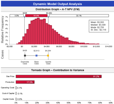
Image from the 4-D Resources article
“In the simple example (to the right), the financial model was more real-world through using input variables and correlation assumptions that reflect historical and projected reality rather than single data estimates that tend towards the most expected value.”
“Additionally, the output data provide greater insight into the variability of outcomes than the static model Downside, Base and Upside cases’ single data estimates did.”
The tornado diagram, shown below the histogram, essentially is another representation of the spider diagram information. ie.e which factors have the biggest impact.
“The dynamic data also facilitated the real option value of the asset in a manner a static model cannot. And the model took less time to build, with less internal relationships to create to make the output trustworthy, given input variables and correlation were set using the @RISK software options. This dynamic modeling approach can be used for all types of financial models.”
To read the full article, follow this link.
Conclusion
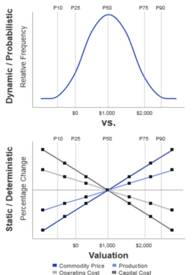
image from 4-D Resources article
Improvements are needed in the way risks are evaluated and explained to mining stakeholders. Improvements are required given increasing complexity in the risks impacting on decision making.
The probabilistic risk evaluation approach described above isn’t new and isn’t that complicated. In fact, it can be very intuitive when undertaken properly.
Probabilistic risk analysis isn’t something that should only be done within the inner sanctums of large mining companies. The approach should filter down to all mining studies and 43-101 reports.
It should ultimately become a best practice or standard part of all mining project economic analyses. The more often the approach is applied, the sooner people will become familiar (and comfortable) with it.
Mining projects can be risky, as demonstrated by the numerous ventures that have derailed. Yet recognition of this risk never seems to be brought to light beforehand.
Essentially all mining projects look the same to outsiders from a risk perspective, when in reality they are not. The mining industry should try to get better in explaining this.
Management understandably have a difficult task in making go/no-go decisions. Financial institutions have similar dilemmas when deciding on whether or not to finance a project. You can read that blog post at this link “Flawed Mining Projects – No Such Thing as Perfection“
Note: You can sign up for the KJK mailing list to get notified when new blogs are posted. Follow me on Twitter at @KJKLtd for updates.


 We likely have all heard the statement that increasing pit wall angles will result in significant cost savings to the mining operation.
 The results of applying the increased inter-ramp angle to each of the four pits is shown in the Bar Chart. Note that the waste reduction is not necessarily the same for each pit. It depends on the specific topography around each pit.
 In general one can typically see four positive outcomes from adopting steeper pit walls. They are as follows:
 4. Pit Crest Location: The steeper wall angles result in a shift in the final pit crest location. The Image shows the impact that the 5 degree steepening had on the crest location for one of the pits in this scenario.
 It is relatively easy to justify spending additional time and money on proper geotechnical investigations and geotechnical monitoring given the potential slope steepening benefits.


 I remember in the late fall of that year, the company had a chance to bid on a larger project in Gros Morne National Park, Newfoundland. So our President, Frank Nolan (he was a brother to Fred Nolan, the infamous land-owner at Oak Island, by the way), decided he wanted to see the site and he chartered a Bell 106 helicopter to fly us there from Deer Lake. It was December (they say “December month” in that province) and when we got close to the Park, we ran into a sudden snow squall.
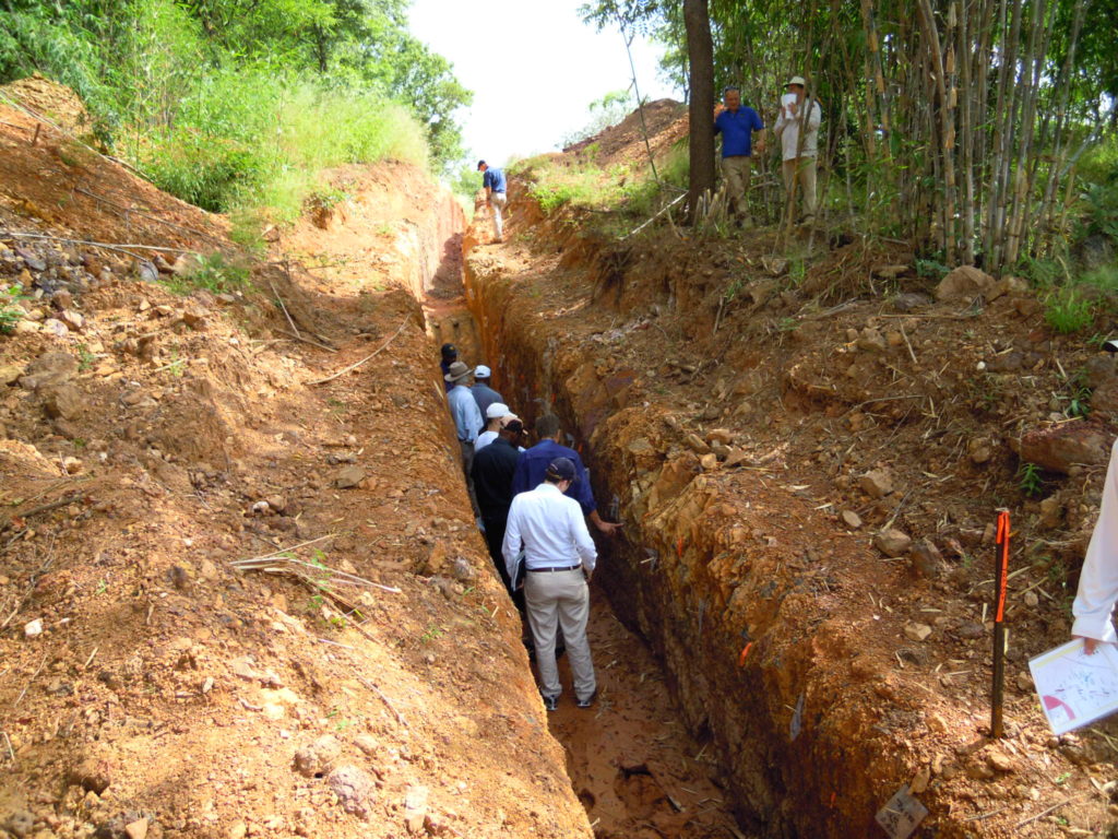
 The QMM field office In Port Dauphin, Madagascar was located near the edge of town, and I typically walked from my lodging to the office each morning when I was there, about the time when school started for the children. Typically I passed dozens and dozens of tiny bamboo huts with corrugated metal roofs, and dirt floors each about 2 meters square.
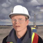 It is one thing to briefly visit a remote project as part of a review team. It is another thing to be there as part of a design team trying to solve a problem and engineer a solution. I know of many engineers and geologists that would have similar work life experiences as part of their careers. However John has taken the initiative to write it all down.
 In today’s world, it is an onerous task to permit, finance, build, and operate a new mine. This is a significant achievement.
 I would suggest that the three reporting categories be used instead of two, described as follows:
 The DRX Drill Hole and Reporting algorithm developed by


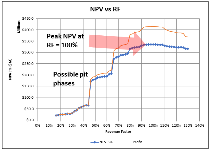 Often in 43-101 technical reports, when it comes to pit optimization, one is presented with the basic “NPV vs Revenue Factor (RF)” curve. That’s it.
 Pit optimization is a approximation process, as I outlined in a prior post titled “
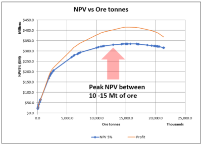


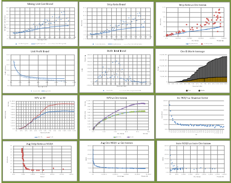 It’s always a good idea to drill down deeper into the optimization output data, even if you don’t intend to present that analysis in a final report. It will help develop an understanding of the nature of the orebody.
 The majority of mining projects tend to consist of either open pit only or underground only operations. However there are instances where the orebody is such that eventually the mine must transition from open pit to underground. Open pit stripping ratios can reach uneconomic levels hence the need for the change in direction.
 There are several reasons why open pit and underground can be considered as two different projects within the same project.
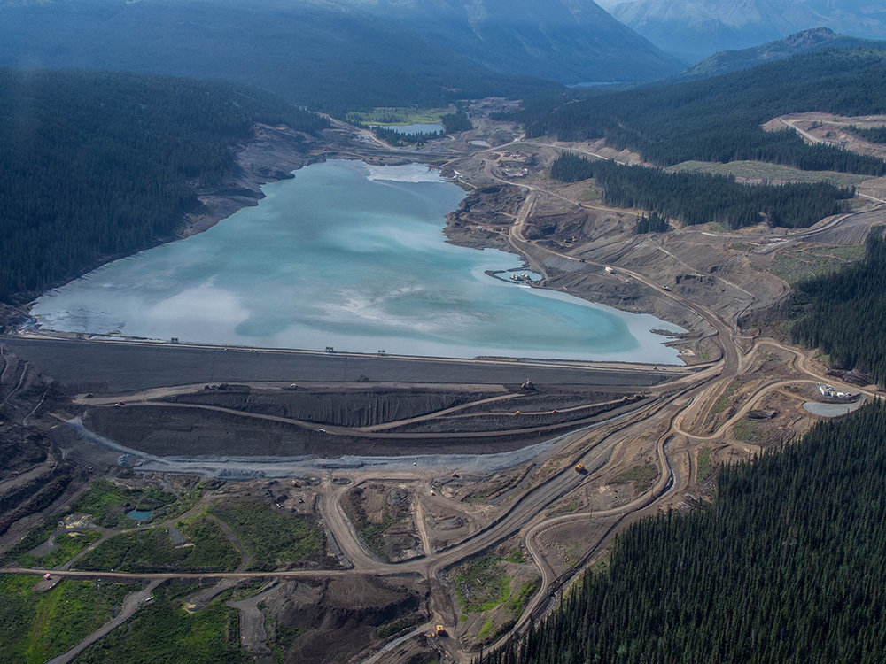 An underground mine that uses a backfilling method will be able to dispose of some tailings underground. Conversely moving towards a larger open pit will require a larger tailings pond, larger waste dumps and overall larger footprint. This helps make the case for underground mining, particularly where surface area is restricted or local communities are anti-open pit.
 Open pit and underground operations will require different skill sets from the perspective of supervision, technical, and operations. Underground mining can be a highly specialized skill while open pit mining is similar to earthworks construction where skilled labour is more readily available globally. Do local people want to learn underground mining skills? Do management teams have the capability and desire to manage both these mining approaches at the same time?
 As you can see from the foregoing discussion, there are a multitude of factors playing off one another when examining the open pit to underground cross-over point. It can be like trying to mesh two different projects together.
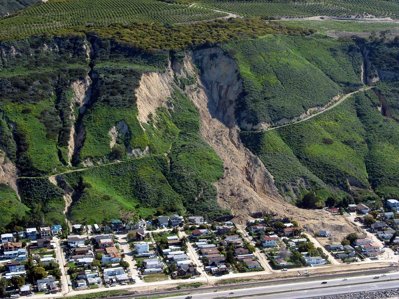 This pessimism training started early in my career while working as a geotechnical engineer. Geotechnical engineers were always looking at failure modes and the potential causes of failure when assessing factors of safety.
 When undertaking a due diligence, particularly for a major company or financier, we are not hired to tell them how great the project is. We are hired to look for fatal flaws, identify poorly based design assumptions or errors and omissions in the technical work. We are mainly looking for negatives or red flags.
 It has been my experience that digging in a data room or speaking with the engineering consultants can reveal issues not identifiable in a 43-101 report. Possibly some of these issues were mentioned or glossed over in the report, but you won’t understand the full extent of the issues until digging deeper.
 My hesitance in investing in some companies unfortunately can be penalizing. I may end up sitting on the sidelines while watching the rising stock price. Junior mining investors tend to be a positive bunch, when combined with good promotion can result in investors piling into a stock.
 Most times the issue is something we couldn’t fully address given the level of study. We might have been forced to make best guess assumptions to move forward. The review engineers will have their opinions about what assumptions they would have used. Typically the common comment is that our assumption is too optimistic and their assumption would have been more conservative or realistic (in their view).
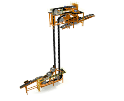 The background information on vertical conveying was provided to me by FKC-Lake Shore, a construction contractor that installs these systems. FKC itself does not fabricate the conveyor hardware. A link to their website is
  The FLEXOWELL®-conveyor system is capable of running both horizontally and vertically, or any angle in between. These conveyors consist of FLEXOWELL®-conveyor belts comprised of 3 components: (i) Cross-rigid belt with steel cord reinforcement; (ii) Corrugated rubber sidewalls; (iii) transverse cleats to prevent material from sliding backwards. They can handle lump sizes varying from powdery material up to 400 mm (16 inch). Material can be raised over 500 metres with reported capacities up to 6,000 tph.
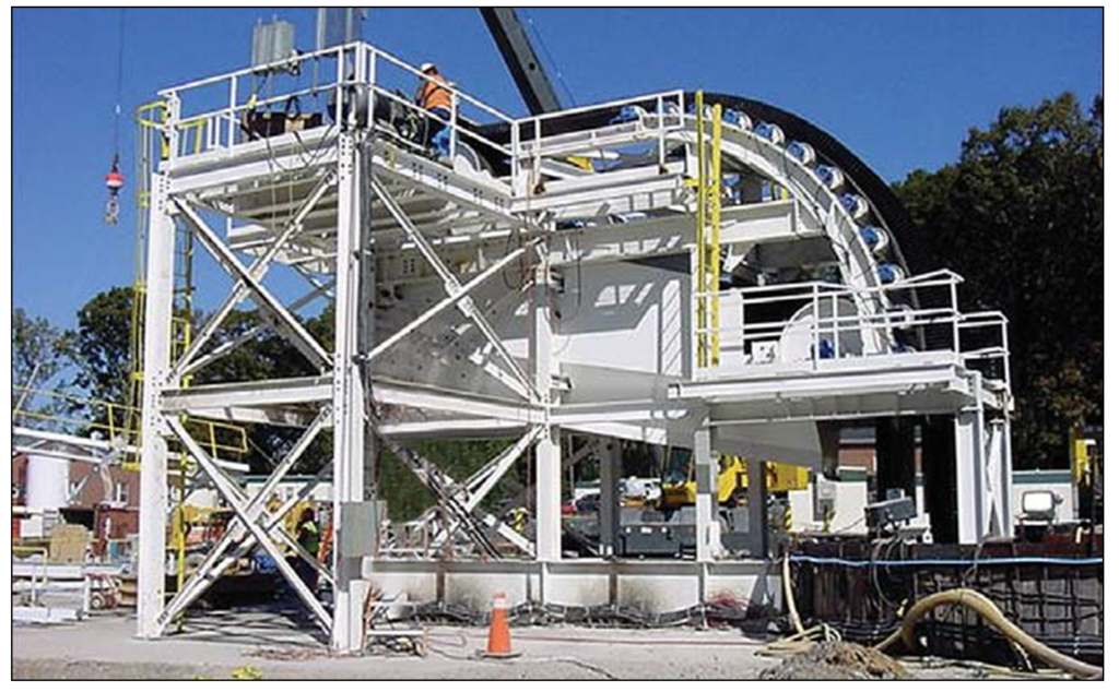 Vendors have evaluated the use of vertical conveying against the use of a conventional vertical shaft hoisting. They report the economic benefits for vertical conveying will be in both capital and operating costs.
 The vendors indicate the conveying system should be able to achieve heights of 700 metres. This may facilitate the use of internal shafts (winzes) to hoist ore from even greater depths in an expanding underground mine. It may be worth a look at your mine.
 While waiting for various third-party due diligences to be completed, the company continue to do exploration drilling. There were still a lot of untested showings on the property and geologists need to stay busy.
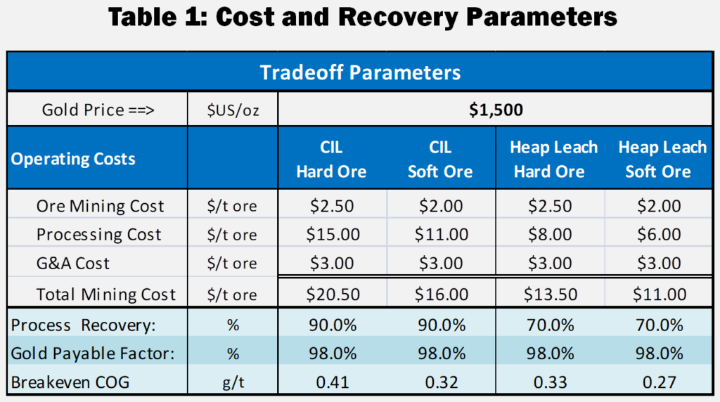 With regards to the Heap Leach PEA, we did not wish to complicate the Feasibility Study by adding a new feed supply to that plant from mixed CIL/HL pits. The heap leach project was therefore considered as a separate satellite operation.
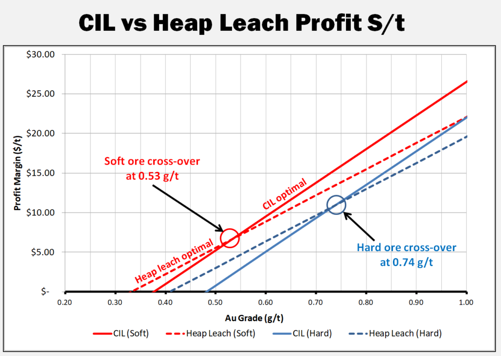 I have updated and simplified the trade-off analysis for this blog. Table 1 provides the costs and recoveries used herein, including increasing the gold price to $1500/oz.
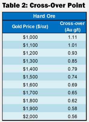 These cross-over points described in Table 2 are relevant only for the costs shown in Table 1 and will be different for each project.