

Every so often I like to comment on issues related to the way the mining industry does things. This is one of those posts.
Currently the mining industry reports their exploration results as either Mineral Resources or Mineral Reserves. In my opinion, these two categories do not adequately reflect the reality of the current mining environment. I would suggest using a three category approach, as will be described below.
The implementation of this approach would not result in any more technical effort. However, it would provide clarity for stakeholders and investors and compare companies on a more equitable basis.
The issue
 In today’s world, it is an onerous task to permit, finance, build, and operate a new mine. This is a significant achievement.
An operating company will be generating revenue and should be recognized for that big step. Hence does it make sense for an operating company to report Mineral Reserves while a junior company that has simply completed a pre-feasibility study to also report Mineral Reserves?
Both companies could report identical Reserves, but those reserves would not be the same thing. One company has built a mine while the other may have spent a few months doing a paper study. One company’s reserves will actually be mined in the foreseeable future while the other company’s project may never see the light of day. Yet both companies are allowed to present the same Mineral Reserves.
As a mine operates, the remaining ore reserves will deplete over time. However, a company can add to their reserves by finding satellite ore bodies or converting inferred material into a higher classification. The net of these adjustments will be reflected in the corporate Mineral Reserve Statement for all their operations.
A company can also increase the corporate Mineral Reserves simply by completing a pre-feasibility or feasibility study on a new project. However, is this a true reflection of the Reserves upon which the company should be evaluated?
Suggestion
 I would suggest that the three reporting categories be used instead of two, described as follows:
1 – Mineral Resources (insitu): This category is the same as the current Mineral Resources being reported according to NI43-101. It is based on reasonable prospects for economic extraction. Hence open pit resources would be reported within an optimized shell and underground reserves within approximate stope shapes. No external dilution or mining criteria would be applied, as is the current approach.
2 – Economic Resources: This would be a new category that would simply be the outcome from a pre-feasibility or feasibility study, which is currently being labelled a “Mineral Reserve”. This Economic Resource would incorporate mining criteria, Measured & Indicated classes only, a mine plan, and an economic analysis. The differentiation from Reserves is because the mine is not built yet.
3 – Mineral Reserves: This highest-level category could be reported only once a mine has reached commercial production. The Economic Resources would automatically convert to Mineral Reserves once production is achieved. As the mine continues to operate, and as new ore sources are identified, the Mineral Reserves would increase / decrease. The Mineral Reserves would represent the remaining ore tonnage at operating mines and only that.
This three-category approach would help separate mine operators from junior development companies. The industry should recognize the difference between companies and projects at different life-cycle stages and that they are not all directly comparable. A junior explorer could be reporting huge reserves, but without a mine being there, should that company be compared to a mine operator that has similar reserves?
This approach would identify situations whereby a company suddenly reports a sizeable increase in Reserves. Is it because they found more ore at an existing operation (a great event) or because they did a paper study on a new project?
As a clarification, if a mine gets placed onto care & maintenance, likely due to poor economics, then the remaining tonnes at the mine would no longer be considered Mineral Reserves and may have to revert to Economic Resources, although even that would be questionable.
Examples
Out of curiosity I randomly selected three companies (Yamana Gold, Eldorado Gold, Alamos Gold) to compare their total Mineral Reserve tonnages based on their operations versus study stage development projects. The results are show in the images below. The percentage of Reserves provided by their producing (P) mines varied and ranged from 14% to 51%. A significant proportion of their Reserves (49% to 86%) are still at the development (D) stage. One or two large study-stage projects can boost the corporate reserves significantly. This is not immediately evident when looking at the total Mineral Reserves being reported.
For most junior miners 100% of their Reserves are still at the study-stage. They should not be able to declare Mineral Reserves and appear on an equal footing with mine operators. Their company should only be comparable to other companies with advanced study-stage projects.
Blog 97 Charts
Blog 97 Charts
Conclusion


 The DRX Drill Hole and Reporting algorithm developed by


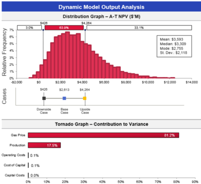

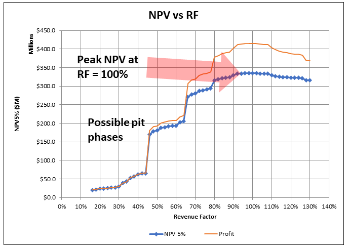 Often in 43-101 technical reports, when it comes to pit optimization, one is presented with the basic “NPV vs Revenue Factor (RF)” curve. That’s it.
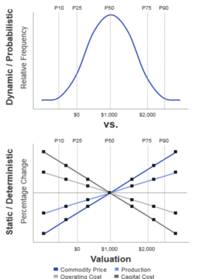
 Pit optimization is a approximation process, as I outlined in a prior post titled “
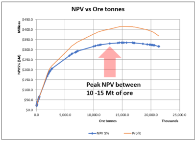


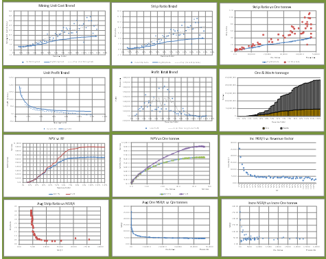 It’s always a good idea to drill down deeper into the optimization output data, even if you don’t intend to present that analysis in a final report. It will help develop an understanding of the nature of the orebody.
 The majority of mining projects tend to consist of either open pit only or underground only operations. However there are instances where the orebody is such that eventually the mine must transition from open pit to underground. Open pit stripping ratios can reach uneconomic levels hence the need for the change in direction.
 There are several reasons why open pit and underground can be considered as two different projects within the same project.
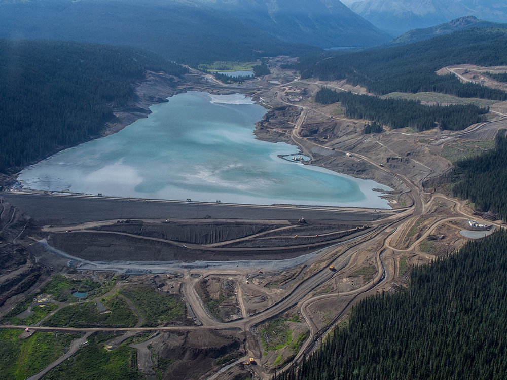 An underground mine that uses a backfilling method will be able to dispose of some tailings underground. Conversely moving towards a larger open pit will require a larger tailings pond, larger waste dumps and overall larger footprint. This helps make the case for underground mining, particularly where surface area is restricted or local communities are anti-open pit.
 Open pit and underground operations will require different skill sets from the perspective of supervision, technical, and operations. Underground mining can be a highly specialized skill while open pit mining is similar to earthworks construction where skilled labour is more readily available globally. Do local people want to learn underground mining skills? Do management teams have the capability and desire to manage both these mining approaches at the same time?
 As you can see from the foregoing discussion, there are a multitude of factors playing off one another when examining the open pit to underground cross-over point. It can be like trying to mesh two different projects together.
 This pessimism training started early in my career while working as a geotechnical engineer. Geotechnical engineers were always looking at failure modes and the potential causes of failure when assessing factors of safety.
 When undertaking a due diligence, particularly for a major company or financier, we are not hired to tell them how great the project is. We are hired to look for fatal flaws, identify poorly based design assumptions or errors and omissions in the technical work. We are mainly looking for negatives or red flags.
 It has been my experience that digging in a data room or speaking with the engineering consultants can reveal issues not identifiable in a 43-101 report. Possibly some of these issues were mentioned or glossed over in the report, but you won’t understand the full extent of the issues until digging deeper.
 My hesitance in investing in some companies unfortunately can be penalizing. I may end up sitting on the sidelines while watching the rising stock price. Junior mining investors tend to be a positive bunch, when combined with good promotion can result in investors piling into a stock.
 Most times the issue is something we couldn’t fully address given the level of study. We might have been forced to make best guess assumptions to move forward. The review engineers will have their opinions about what assumptions they would have used. Typically the common comment is that our assumption is too optimistic and their assumption would have been more conservative or realistic (in their view).
 The background information on vertical conveying was provided to me by FKC-Lake Shore, a construction contractor that installs these systems. FKC itself does not fabricate the conveyor hardware. A link to their website is
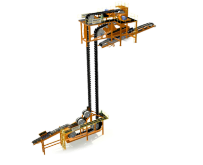
  The FLEXOWELL®-conveyor system is capable of running both horizontally and vertically, or any angle in between. These conveyors consist of FLEXOWELL®-conveyor belts comprised of 3 components: (i) Cross-rigid belt with steel cord reinforcement; (ii) Corrugated rubber sidewalls; (iii) transverse cleats to prevent material from sliding backwards. They can handle lump sizes varying from powdery material up to 400 mm (16 inch). Material can be raised over 500 metres with reported capacities up to 6,000 tph.
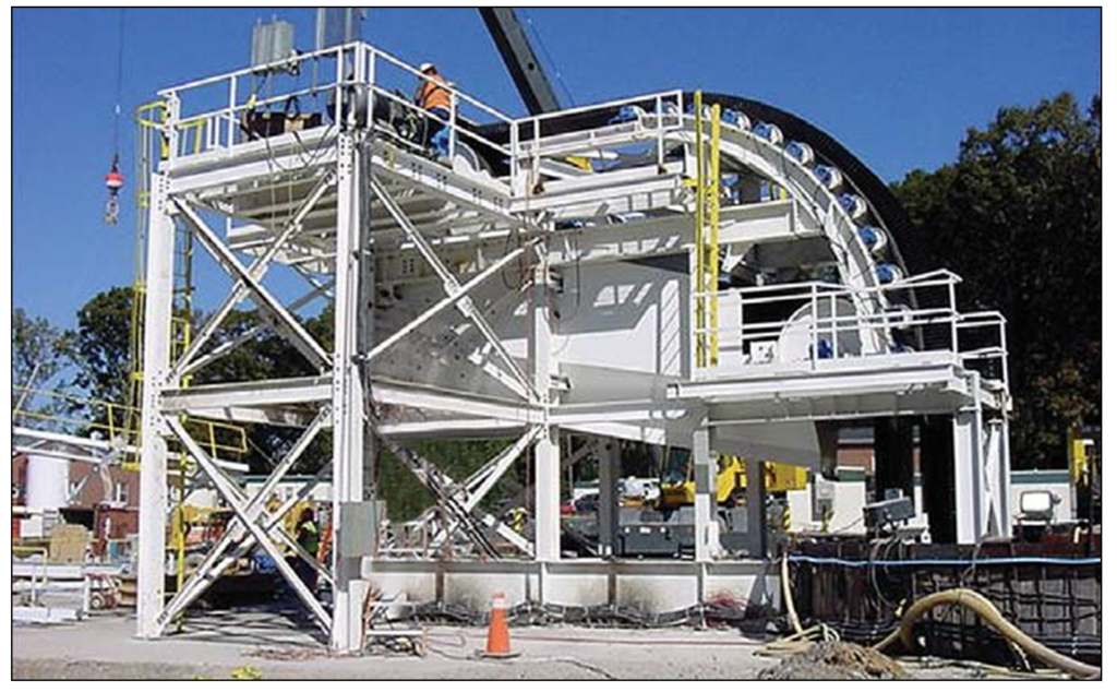 Vendors have evaluated the use of vertical conveying against the use of a conventional vertical shaft hoisting. They report the economic benefits for vertical conveying will be in both capital and operating costs.
 The vendors indicate the conveying system should be able to achieve heights of 700 metres. This may facilitate the use of internal shafts (winzes) to hoist ore from even greater depths in an expanding underground mine. It may be worth a look at your mine.
 While waiting for various third-party due diligences to be completed, the company continue to do exploration drilling. There were still a lot of untested showings on the property and geologists need to stay busy.
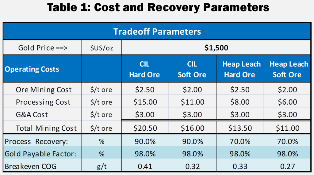 With regards to the Heap Leach PEA, we did not wish to complicate the Feasibility Study by adding a new feed supply to that plant from mixed CIL/HL pits. The heap leach project was therefore considered as a separate satellite operation.
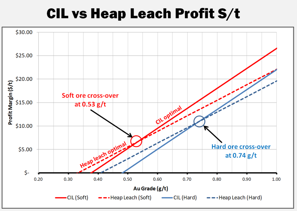 I have updated and simplified the trade-off analysis for this blog. Table 1 provides the costs and recoveries used herein, including increasing the gold price to $1500/oz.
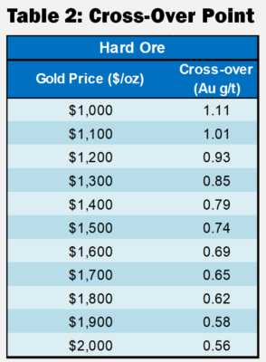 These cross-over points described in Table 2 are relevant only for the costs shown in Table 1 and will be different for each project.
 Normally I don’t write about mining stock markets, preferring instead to focus on technical matters. However I have seen some recent discussions on Twitter about stock price trends. For every stock there are a wide range of price expectations. Ultimately some of the expectations and realizations can be linked back to the Lassonde Curve.
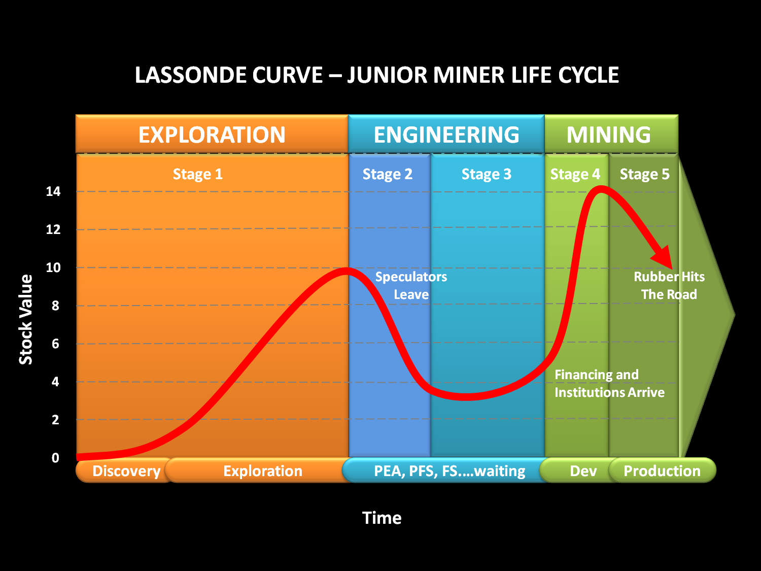
 Stage 5 is the start-up and commercial production period, possibly nerve-racking for some investors. This is where the rubber hits the road. The stock price can fall if milled grades, operating costs, or production rates are not as expected.
 Some corporate presentations will highlight the Lassonde Curve, particularly when they are rising in Stage 1. You are less likely to see the curve presented when they are rolling along in Stages 2 or 3.
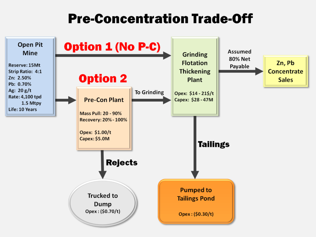
 Concentrate handling systems may not differ much between model options since roughly the same amount of final concentrate is (hopefully) generated.
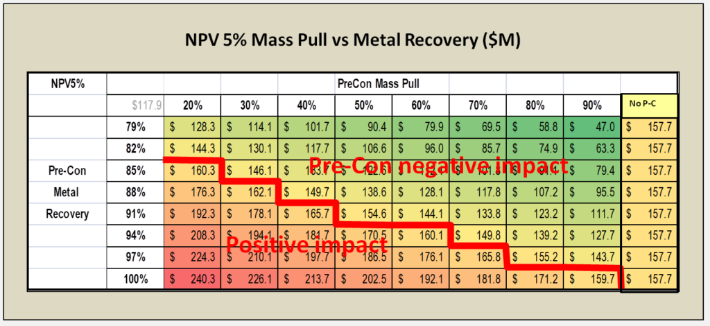
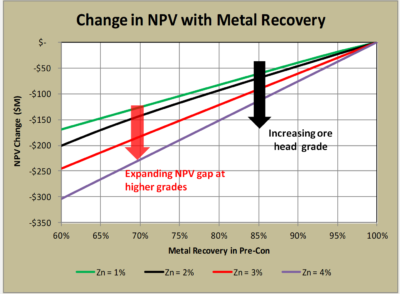 4. The head grade of the deposit also determines how economically risky pre-concentration might be. In higher grade ore bodies, the negative impact of any metal loss in pre-concentration may be offset by accepting higher cost for grinding (see chart on the right).