As a mining engineer, I am not usually called in to review a project that is still at the exploration stage. This is normally the domain of the geologist. However from time to time I have an interest in better understanding the potential of an early stage mining project. This could be on behalf of a client, for investing purposes, or just for personal curiosity.
 At the exploration stage one only has drill interval data from news releases to examine. A resource estimate may still be unavailable.
The drill data can consist of long intervals of low grade or short intervals of high grade and everything in between. What does it all mean and what can it tell you?
The following describes an approach I use for examining early stage gold deposits. The logic can be expanded to other metals but would take more effort.
My focus is on gold because it has been the predominant deposit of interest over the last few years, and it is simpler to analyze quickly.
We All Like Scatter Plots
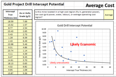
My approach relies on a scatter plot to visual examine the distribution of interval thicknesses and gold grades. Where these data points cluster or how they are distributed can provide some prediction on the overall economic potential of a project. Its not a guarantee, but only an indicator.
I try to group the analysis into potential open pit intervals (0 to 200 metres from surface) and potential underground (deeper than 200m) intervals. This is because a 20m wide interval grading 2.0 g/t is of economic interest when near surface, however of less interest if occurring at a 300m depth.
 Using information from a news release, I create a two column Excel table of highlighted intervals and assay grades. The nice thing about using intervals is that the company has provided their view of the mineable widths.
If one is provided with raw 1-metre assay data you would have to make that decision, which can be a significant task. The company has already helped make those decisions.
Normally I tend to use the highlighted sub-intervals and not the main intervals since issues with grade smoothing can occur.
A large interval containing multiple high grade sub-intervals may see some grade smoothing.This happens if the grade between sub-intervals is very low grade or even waste. It takes a fair bit of effort to assess this for each drill hole, hence it is easier to work with the sub-intervals.
NOTE: Due to changes with Google security protocols, the online calculators have been take offline until a resolution can be implemented.
I have an online calculator (Drill Intercept Calculator) that lets you assess if grade smoothing is occurring.
When inputting the interval thickness, I prefer to use the true thickness and not the interval length. If the assay information does not specify true thicknesses, then I simply multiple the interval length by 0.70 to try to accommodate some possible difference in width. Its all subjective.
The assays can consist of Au (g/t) or AuEq (g/t) if more metals are present. If very high grades are encountered (greater than 10 g/t) I simply input 9.9 g/t into the Excel table so they fit onto my scatter plot. Extremely high grades can be sporadic and localized anyhow.
Finally I need to decide whether the project is located in a region of high operating cost, low cost or about average costs. High costs could be with a fly in/ fly out, camp operation, with diesel power, and seasonal access.
A low cost operation could be in temperate climate, with good access to local infrastructure, water, labour, and grid power. An average operation would be somewhere in between the two. Its just a gut feel.
Results
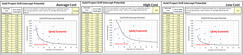
The following charts describe how it works, using randomly generated dummy assay data in this example.
In the Average cost scenario (left chart) the points are equally scattered both above and below the Likely Economic line. As one moves to a high-cost situation (middle chart) the curve moves upwards and more drill intervals now fall below the economic line.
This would give me an unfavorable impression of the project. The third graph is the Low-Cost scenario and one can see that more assays are now above the line. Hence the same project located in a different region would yield a different economic impression.
The economic boundaries (dashed lines) presented in the plots are based on my personal experience and biases. Other people may have different criteria to define what they would view as economic and uneconomic intervals.
Conclusion
There is not much that a layperson person can do with the multitude of exploration data provided in corporate news releases. However, by aggregating the data one can get a sense of where a gold project positions itself economically. The more data points available, the more that one can gather from the plot.
One should prepare separate plots for shallow and deep mineralization or for different zones and deposits on a property rather than aggregate everything together.
It may be possible to undertake a similar analysis with different commodities if one can summarize the assays into a single equivalent value or NSR dollar value. Unfortunately, exploration news releases don’t often include the poly-metallic interval equivalent grade or NSR value. Calculating these manually would add an extra step in the process, however it can be done.
If you want to try out the concept, I have posted the online spreadsheet to my website at the link Drill Intercept Potential where you can input Au exploration data of interest. Unfortunately, you cannot save your input data so it’s a one time event. Anyone can do this – its not rocket science.
Let me know your thoughts, suggestions, or other ways to play with news release data.
If your project contains metals other than gold, then the rock (or ore) value will be based on the revenue from a combination of metals. How to approach this in discussed in another blog post titled “Ore Value Calculator – What’s My Ore Worth?“
Great Bear Resources Example
Interesting the Great Bear Resources website allows one to download a data file with all their exploration intervals. I have not seen another company provide this level of transparency. I download their data file of over 1300 intervals and sub-divided them into major intervals and sub-intervals (more ore less). The two plots below show the outcome.
The graph on the left is the sub-intervals showing that many points are above the “economic” line. There are numerous data points along the top axis, indicating many sub-intervals at >10 g/t at widths ranging from 1 to 15 metres. The graph on the right shows the major intervals. While there are still many along the top axis, there are now more along the 40m width but at grades ranging from 1 g.t to 6 g/t.
One would surmise from these plots that overall there are many intervals above the line in the economic zone, showing the potential of the project. It also shows that GBR have encountered many intervals likely sub-economic, but that’s the exploration game.

Great Bear Resources data
Examining polymetallic drill results in a similar manner isn’t as simple as this. The mutiple metals of interest make the calaculations a bit more complex. Another blog post discusses the approach I use for polymetallic, at this this link “Polymetallic Drill Results – Interesting or Not?“
Note: You can sign up for the KJK mailing list to get notified when new blogs are posted. Follow me on Twitter at @KJKLtd for updates and insights.


 The DRX Drill Hole and Reporting algorithm developed by Objectivity.ca uses artificial intelligence to optimize the infill drilling layout. It intends to match the QP/CP constraints with corporate/project objectives.


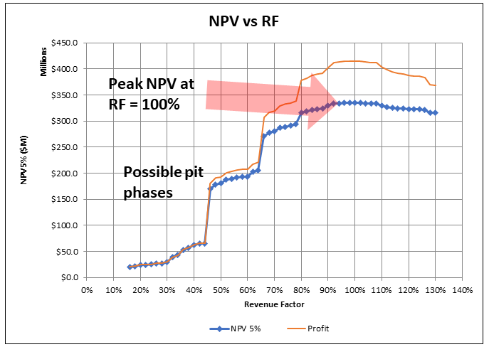 Often in 43-101 technical reports, when it comes to pit optimization, one is presented with the basic “NPV vs Revenue Factor (RF)” curve. That’s it.
 Pit optimization is a approximation process, as I outlined in a prior post titled “
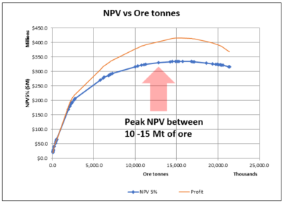


 It’s always a good idea to drill down deeper into the optimization output data, even if you don’t intend to present that analysis in a final report. It will help develop an understanding of the nature of the orebody.
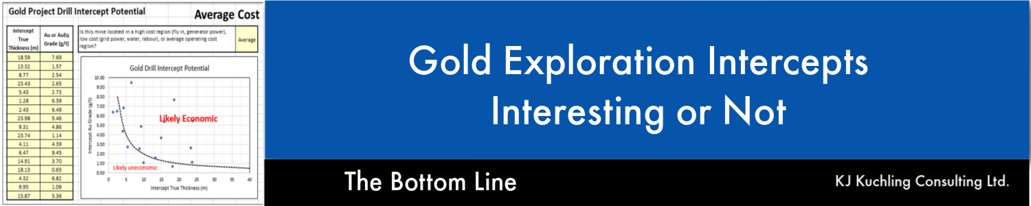


 The majority of mining projects tend to consist of either open pit only or underground only operations. However there are instances where the orebody is such that eventually the mine must transition from open pit to underground. Open pit stripping ratios can reach uneconomic levels hence the need for the change in direction.
 There are several reasons why open pit and underground can be considered as two different projects within the same project.
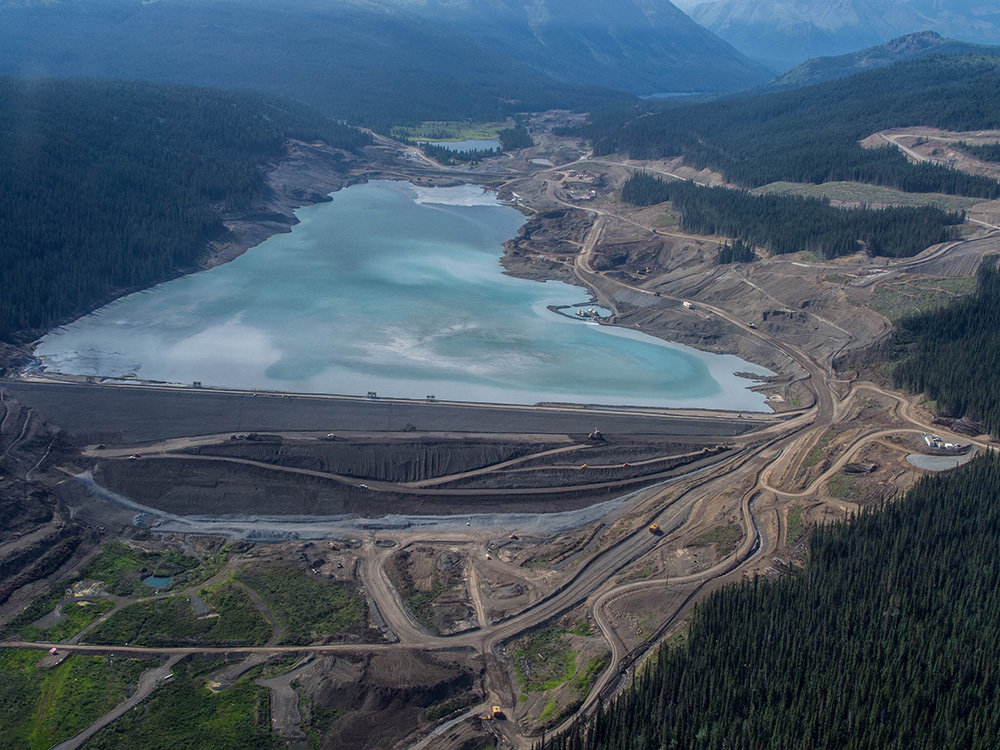 An underground mine that uses a backfilling method will be able to dispose of some tailings underground. Conversely moving towards a larger open pit will require a larger tailings pond, larger waste dumps and overall larger footprint. This helps make the case for underground mining, particularly where surface area is restricted or local communities are anti-open pit.
 Open pit and underground operations will require different skill sets from the perspective of supervision, technical, and operations. Underground mining can be a highly specialized skill while open pit mining is similar to earthworks construction where skilled labour is more readily available globally. Do local people want to learn underground mining skills? Do management teams have the capability and desire to manage both these mining approaches at the same time?
 As you can see from the foregoing discussion, there are a multitude of factors playing off one another when examining the open pit to underground cross-over point. It can be like trying to mesh two different projects together.
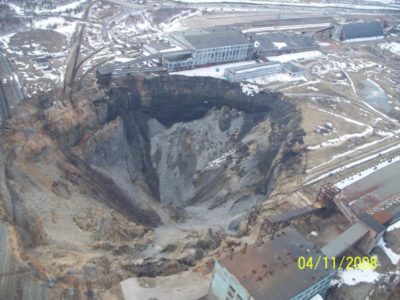
 This pessimism training started early in my career while working as a geotechnical engineer. Geotechnical engineers were always looking at failure modes and the potential causes of failure when assessing factors of safety.
 When undertaking a due diligence, particularly for a major company or financier, we are not hired to tell them how great the project is. We are hired to look for fatal flaws, identify poorly based design assumptions or errors and omissions in the technical work. We are mainly looking for negatives or red flags.
 It has been my experience that digging in a data room or speaking with the engineering consultants can reveal issues not identifiable in a 43-101 report. Possibly some of these issues were mentioned or glossed over in the report, but you won’t understand the full extent of the issues until digging deeper.
 My hesitance in investing in some companies unfortunately can be penalizing. I may end up sitting on the sidelines while watching the rising stock price. Junior mining investors tend to be a positive bunch, when combined with good promotion can result in investors piling into a stock.
 Most times the issue is something we couldn’t fully address given the level of study. We might have been forced to make best guess assumptions to move forward. The review engineers will have their opinions about what assumptions they would have used. Typically the common comment is that our assumption is too optimistic and their assumption would have been more conservative or realistic (in their view).
 The background information on vertical conveying was provided to me by FKC-Lake Shore, a construction contractor that installs these systems. FKC itself does not fabricate the conveyor hardware. A link to their website is
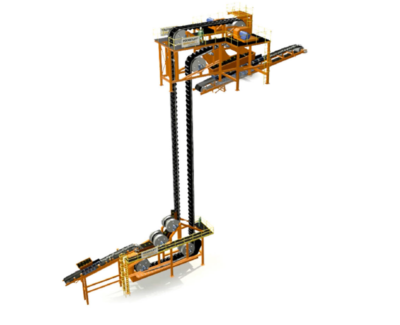
  The FLEXOWELL®-conveyor system is capable of running both horizontally and vertically, or any angle in between. These conveyors consist of FLEXOWELL®-conveyor belts comprised of 3 components: (i) Cross-rigid belt with steel cord reinforcement; (ii) Corrugated rubber sidewalls; (iii) transverse cleats to prevent material from sliding backwards. They can handle lump sizes varying from powdery material up to 400 mm (16 inch). Material can be raised over 500 metres with reported capacities up to 6,000 tph.
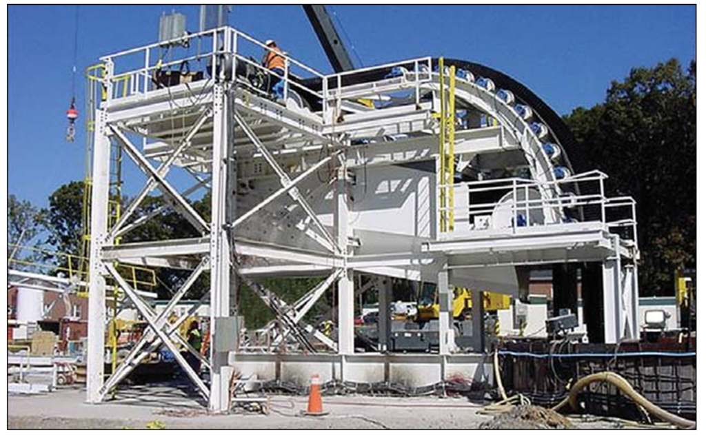 Vendors have evaluated the use of vertical conveying against the use of a conventional vertical shaft hoisting. They report the economic benefits for vertical conveying will be in both capital and operating costs.
 The vendors indicate the conveying system should be able to achieve heights of 700 metres. This may facilitate the use of internal shafts (winzes) to hoist ore from even greater depths in an expanding underground mine. It may be worth a look at your mine.
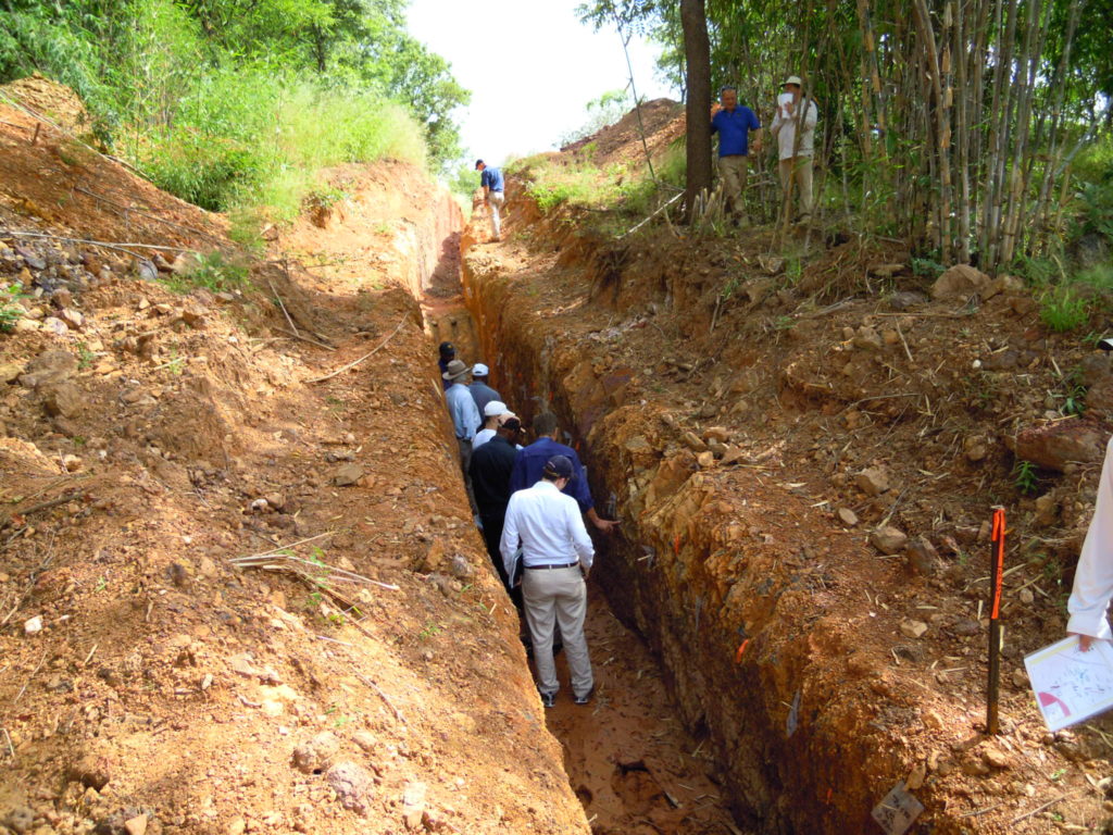
 Based on my own career, mining has definitely provided me with a chance to travel the world. It will also help anyone overcome their fear of travel. One will also learn that both international and domestic travel can be as equally rewarding. There is nothing wrong with learning more about your own country.

 Business travel has always been one of the best parts of my mining career. I can remember the details about a lot of the travel that I did. Unfortunately the project details themselves will blur with those of other projects.
 While waiting for various third-party due diligences to be completed, the company continue to do exploration drilling. There were still a lot of untested showings on the property and geologists need to stay busy.
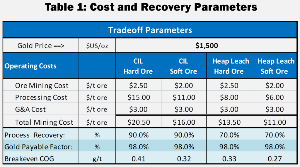 With regards to the Heap Leach PEA, we did not wish to complicate the Feasibility Study by adding a new feed supply to that plant from mixed CIL/HL pits. The heap leach project was therefore considered as a separate satellite operation.
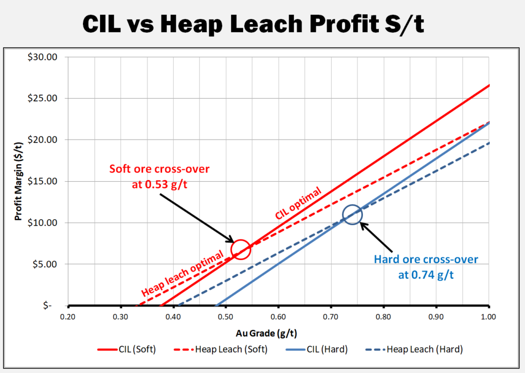 I have updated and simplified the trade-off analysis for this blog. Table 1 provides the costs and recoveries used herein, including increasing the gold price to $1500/oz.
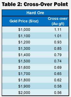 These cross-over points described in Table 2 are relevant only for the costs shown in Table 1 and will be different for each project.